Eventually, You May Need to Know How to Dissect a Notebook Page

We discussed in the CWPK #10 installment of this Cooking with Python and KBpedia series the role of Jupyter Notebook pages to document this entire plan. The reason we are using electronic notebooks is because, from this point forward, we will be following the discipline of literate programming. Literate programming is a style of coding introduced by Donald Knuth to combine coding statements with language narratives about what the code is doing and how it works. The paradigm, and thus electronic notebooks, is popular with data scientists because activities like machine learning also require data processing or cleaning and multiple tests with varying parameters in order to dial-in resulting models. The interactive notebook paradigm, combined with the idea of the scientist’s lab notebook, is a powerful way to instruct programming and data science.
In this installment we will dissect a Jupyter Notebook page and how we write the narrative portions in a lightweight mark-up language known as Markdown. Actually, Markdown is more of a loose affiliation of related formats, with lack of standardization posing some challenges to its use. In the next installment we will provide recipes for keeping your Markdown clean and for integrating notebook pages into your workflows and directory structures.
We first showed a Jupyter Notebook page in Figure 5 of CWPK #10. Review that installment now, make sure you have a CWPK notebook page (*.ipynb) somewhere on your machine, go to the directory where it is stored (remember that needs to be beneath the root directory you set in CWPK #10), and then bring up a command window. We’ll start up Jupyter Notebook first:
$ jupyter notebookAssuming you are using this current notebook page as your example, your screen should look like this one. To confirm our notebook is active, type in our earlier ‘Hello KBpedia!‘ statement:
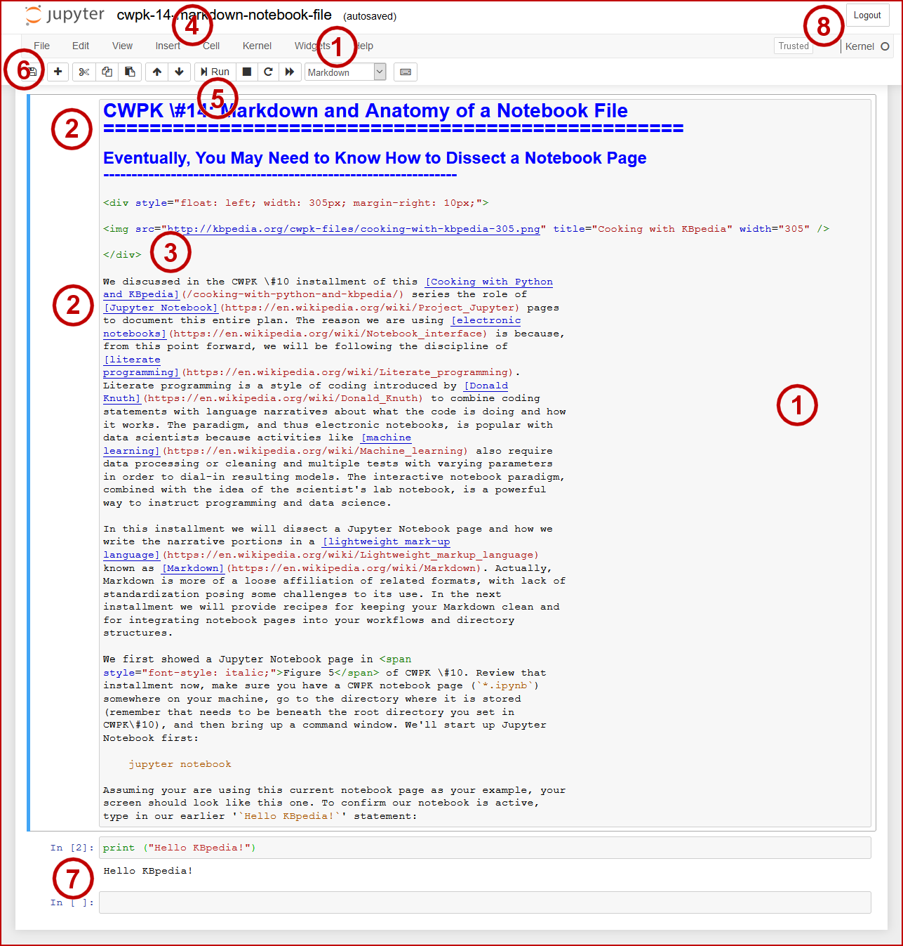
print ("Hello KBpedia!")Now, scroll up to the top of this page and double-click anywhere in the area where the intro narrative is. You should get a screen like the one below, which I have annotated to point out some aspects of the interactive notebook page:

We can see that the active area on the page, what is known as a “cell” contains plain text (1). Also note that the dropdown menu in the header (1) tells us the cell is of the ‘Markdown’ type. There are multiple types of cells, but throughout this series we will be concentrating on the two main ones: Markdown for formatting narratives, and Code for entering and testing our scripts. Recall that Markdown uses plain text rather than embedded tags (as in HTML, for example) (2). We have conventions for designating headings (2) or links with URLs and link text (2). Most common page or text formatting such as bullets or italics or emphasized text or images have a plain text convention associated with them. In this instance, we are using the Pandoc flavor of Markdown. But, also notice, that we can mix many HTML elements (3) into our Markdown text to accomplish more nuanced markup. In this case, we as using the HTML <div> tag to convey style and placement information for our header with its logo.
As we open or close cells, new cells appear for entry at the bottom of our page. We can also manage these cells by inserting above or below or deleting them via two of the menu options (4). To edit, we either double-click in a Markdown cell or enter directly into a Code cell. When have finished our changes, we can see the effect via the Run button (5) or Cell option (4), including to run all cells (the complete page) or selected cells. But be careful! While we can do much entry and modifications with Markdown cells, this application is not like a standard text editor. We can get instant feedback on our modifications, but it is different to Save files as checkpoints (6) and changing file names is not possible from within the notebook, where we must use the file system. We can also have multiple cells unevaluated at a given time (7). We may also choose among multiple kernals (different languages or versions, including R and others). Many of these features we will not use in this series; the resources at the end of this article provide additional links to learn more about notebooks.
To learn more about Markdown, let me recommend two terrific resources. The first is directly relevant to Jupyter Notebook, the second is for a very useful Markdown format:
When you are done working on your notebook, you can save the notebook using Widgets → Save Notebook Widgets State OR File → Save and Checkpoint and then File → Close and Halt. (You may also Logout (8), but make sure you have saved in advance.) Depending on your sequence, you may exit to the command window. If so, and the system is still running in the background, pick Ctrl+c to quit the application and return to the command window prompt.
Should you want to convert your notebook to a Web page (*.html), you may use nbconvert at the command prompt when you are out of Jupyter Notebook. For the notebook file we have been using for this example, the command is (assuming you are in the same directory as the notebook file):
$ jupyter nbconvert --to html cwpk-14-markdown-notebook-file.ipynbThis command will write out a large HTML page (large because it embeds all style information). This version pretty faithfully captures the exact look of the application on screen. See the nbconvert documentation for further details. Alternatively, you may export the notebook directly by picking File → Download as → HTML (.html). Then, save to your standard download location.
We will learn more about these saving options and ways to improve file size and faithful rendering in the next installment.
Important note: as of the forthcoming CWPK #16 installment, we will begin to distribute Jupyter Notebook files with the publication of each installment. Further, even though early installments in this series had no interactivity, we will also re-published them as notebook files. From this point forward all new installments will include a Notebook file. Check out CWPK #16 when it is published for more details.
More Resources
- Jupyter Notebook Users Manual from Bryn Mawr College (nice
*.ipynbversion) - The Ultimate User’s Guide to Jupyter Notebooks
- Tutorial: Advanced Jupyter Notebooks
- Jupyter Notebook Extensions
- Advanced Jupyter Notebook Tricks — Part I
- Jupiter Notebook Tips & Tricks
- Making Publication-ready Python Notebooks.
*.ipynb file. It may take a bit of time for the interactive option to load.


