 Part II of The Value of Connecting Things: Big Structure Improves Big Data by Orders of Magnitude
Yesterday in the first part of this series we raised the important question of how to value connections made between data. At the Big Data scales represented, we prepared a Basic Facts case of up to 2 billion assertions. We are using asserted “facts” as our value proxy. We’ll talk more about value and caveats in the third part of our series, tomorrow.
We saw that early estimates of network effects, such as Metcalfe’s law, overestimate value at scale. We looked at Zipf’s law as a means to capture the diminishing value of connections given the distance between facts. In today’s article we will focus on these factors of interaction and potential value in the specific context of knowledge graphs. Knowledge graphs are Big Structure representations that capture the schematics, concepts and measures in any given knowledge domain (that is, any domain of human activity).
Since I first tried to address the value of knowledge networks some five years ago [1], I have been disturbed about a couple of things [2]. First, I felt that the exponential or geometric bases for estimating the value of information connections were not correct, both because they fail at scale and they don’t discriminate that some connections work and are more important, while others are trivial or don’t work. Capturing this law of diminishing value in a context that makes sense for knowledge bases was, I felt, the key to answering the value riddle.
I believe we have now, in this series, provided a compelling basis for solving that riddle, which also points the way to further improvements. This assertion is an exciting statement, in that we now may have a quantitative basis in hand for determining where and how to spend our monies for Big Data and Big Structure initiatives. Such quantitative tools are a huge boon to bring analytic rigor to the data collection and integration challenge.
This article shows that adding connections (“Big Structure“) at Big Data scales can increase the value of enterprise information from one (ten) to three (thousands) orders of magnitude. The magnitude of the value scales linearly with each added structure (attribute). These value multipliers from adding Big Structure are a tremendously cost-effective addition to standard data wrangling efforts.
The Value of Knowledge Graphs (VKG) Formulation
The recognition of the need for a law of diminishing returns to reflect the distance between facts or assertions is a central argument in the Briscoe-Odlyzko-Tilly formulation (see [3] directly, and the prior Part I discussion). Not all information is connected, and not all connected information is of equivalent worth. The implied question in these statements, however, is how to capture those differences?
The B-O-T (or sometimes, O-T) formulation does not choose a bad starting proxy for this diminishment law. Zipf’s law reflects many observed distributions in human objects, roughly equivalant to power law, Pareto (“80:20”) distributions or n log (n) diminishing returns with long-tail characteristics. Examples include Internet distributions (such as popularity of Web sites or search terms), human language distributions, income rankings, population distributions, etc. There is no question that Zipf’s law distributions are common and frequent.
The only problem with picking the Zipf’s law basis, however, is that there was absolutely no evidence that such occurred for information networks or knowledge graphs. Zipf’s law distributions tend to be statements across single types for a single attribute distribution. Graphs, we can safely say, are anything but this distribution. Connections and multiple types are the rule, not the exception.
So, maybe the B-O-T formulation was correct, and maybe it was not. There was no empirical evidence to support this assertion for knowledge graphs. And, there did not appear to be a compelling logic argument for relating Zipf’s law to graphs other than they are artifacts of human endeavor.
My discomfort in adopting this arbitrary B-O-T basis, even though solidly embedded in human experience, caused me to seek alternative ideas and explanations, but also ones that fulfilled the key structural insights of diminishing returns and non-equivalent assertions that were the focal points of B-O-T, all within a graph context.
The Starting Basis
The breakthough occurred when I discovered an obscure, un-cited paper by Yaakov Stein [4]. Stein, a network and signals processing researcher of the first rank [4], wrote his paper as a means to understand and quantify his experience of joining LinkedIn and expanding his network. He began without an account and documented his experience as he joined and expanded his network of contacts on LinkedIn. He charted direct links, and then meticulously looked at and recorded secondary and tertiary links.
His formulation recognized that the value to an individual user equaled raising the access to the entire network (1) for that user plus the diminishing benefit represented by the participating graph’s other participants as measured by average degree of separation (d). d is an inherent measure of the graph type.
Though his context was a social network, the basic observation obtains: relations diminish by distance within a graph, with average link distance (directly related to degree of separation) being the key relevance metric. Connected “facts” or “friends” is essentially the same thing. It is all about what is shared amongst graph nodes.
The usefulness of this approach is that it grounds the multiplier effect in an inherent characteristic of the source graph, its average degree of separation [5]. Like Zipf’s law, the degree of separation is a distance measure, but one grounded specifically in graphs. Here is the Stein formulation:

A graph with a degree of separation of 4, then, would exhibit a network-wide power factor of 5/4 (4/4 plus 1/4).
The Viking Algorithm
As applied to knowledge graphs, however, this formulation still has two problems. The first minor one is that the degree of separation parameter should be D (the average across structure) rather than d. The second substantive one is that a correction factor needs to be included that accounts for the probability that an assertion may be false. This factor, F, is 1 – the measured error rate.
The resulting algorithm we term the Value of Knowledge Graph formulation, or the VKG (Viking) algorithm. It is expressed like this:

F is meant to be analogous to F-measure, the combined precision and recall statistic for information retrieval and NLP tasks. F in the case of the Viking algorithm is also meant to be a combined statistic that represents the “accuracy” (verifiable truthfulness) of statements asserted in the graph. F is essentially an estimated value for the residual falsity for the average statement in a graph, after removal of all assertions that do not meet existing coherency, consistency or completeness tests. F is determined by sampling statements across the graph and manually testing for truthfulness (or in a logical sense, validity given the existing statements in the graph). An F of 1 signifies complete truthfulness (accuracy); an F of 0 represents complete falsity [6].
Viking in Relation to Other Network Estimators
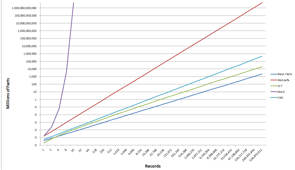
Now, with this explanation of basis, we can again look at the value of the Viking (VKG) algorithm in comparison to those discussed in the first part of this series. Again on a logarithmic scale, here are those results:
Excluding the exponential and geometric multipliers (namely, the “laws” of Metcalfe and Reed) in the top two curves, this shows the Viking (VKG) algorithm to have higher value than the B-O-T (O-T) algorithm, both of which are considerably higher than the Basic Facts. However, because the Figure 1 above has a logarithmic scale, these differences are harder to discern.
Viking Benefits Over the Basic Facts
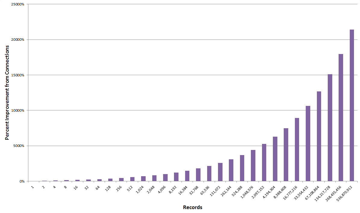
Now corrected with our assumed F factor, we can begin to tease out the value benefits of connecting “facts” versus the unconnected Basic Facts. As with any logarithmic function, we see that the value benefits from connections increase in a growing manner at larger scales. For example, as Figure 2 shows below, at a level of 1000 records, the benefits from connections are 7x greater than unconnected data. By the time the scale grows to 1 million or 500 million records, the value benefits of connections grows to 44x to 215x, respectively:
Benefits from connections increase as a power function at increasing scales.
Setting the VKG Factor D
But the potential value of connectedness is also a function of the general degree of information separation for the given domain. We are still in the early phases of gathering statistics for such things, but the table below summarizes what is known about the “standard” level of connectivity in various domains and applications. Note, in general, most any knowledge graph would have a D factor ranging from 2 to 8:
| Category | Degrees of Separation (D) | Notes |
| Food webs | ~ 2 | [7] |
| Genetic differences | ~ 3 | [8] |
| ~ 3 | [4] | |
| 3.435 – 4.67 | [9] | |
| 3.74 | [10] | |
| Potential research collaborators | ~ 4 | [11] |
| UMBEL | ~ 5.2 | [12] |
| Social networks (general) | ~ 6 | |
| Mobile ad hoc networks | ~ 7 | [13] |
| Small-world networks (max) | ~ 8 | [14] |
More tightly linked, cohesive domains tend to have the lower degrees of separation. It is also interesting to note that some social networks, like Twitter and Facebook, are also able to lower degrees of separation (in comparison to their nominal “social network” benchmark) by virtue of the nature of their service.
As experience is gained and with more research, I expect more estimates and more refined ones. Depending on the nature of the domain at hand, it should then be possible to pick the closest analog to use in the Viking valuation algorithm. Nonetheless, we already have a range and respective values to provide meaningful value estimates today.
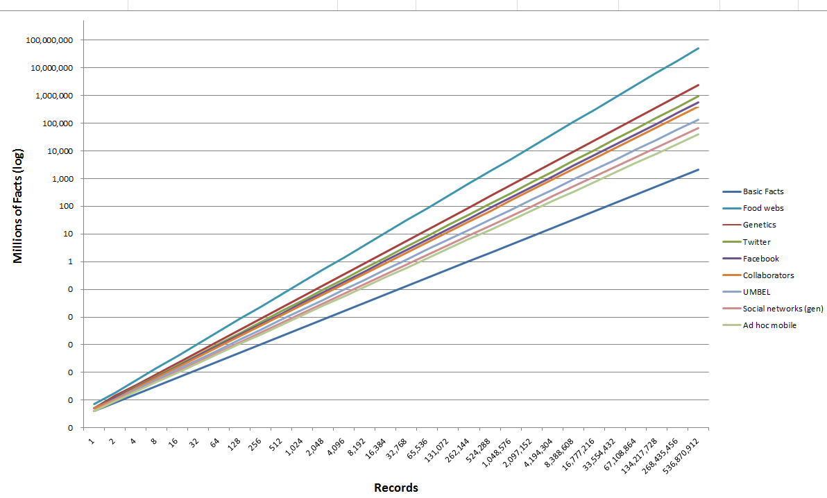
Using the values in Table 1, we are thus able to plot the effects (again, log scale) of these various degrees of separation in terms of the “fact” assertions that can be made for our Big Data test dataset:
At the nominal Big Data scales of 100,000 and 1,000,000 records, the value of data connections in comparison to the unconnected Basic Facts case shows these following value improvement multipliers:
| Domain | 100,000 Records | 1,000,000 Records |
| Food webs | 203x | 611x |
| Genetic differences | 38x | 84x |
| 23x | 46x | |
| 17x | 33x | |
| Potential research collaborators | 14x | 26x |
| UMBEL | 8x | 12x |
| Social networks (general) | 5x | 8x |
| Mobile ad hoc networks | 3x | 5x |
Of course, our “Big Data Example” from Part I was silent about the exact nature of its knowledge graph. Based on empircial experience to date, the benefits from connecting data that was previously unconnected should fall somewhere within the limits of Table 2. Even at rather low scales and more loosely-connected domains, the value improvements in making connections with data is many-fold. At larger scales for tighter networks, the multipliers can become astounding.
Adding Structure to the Underlying Data
Another implication that the Viking algorithm allows us to test is the comparative benefit from adding structure to our datasets. Actually, “adding structure” is not strictly correct; it is “structurizing” the data via characterizations, attributes and categorizations. Of course, not all structure is created equal. Assigning or classifying our records into types, for example, applies to all records across the datasets and provides powerful cross-record linkages. Adding annotations or metadata to single records provides much lower benefits.
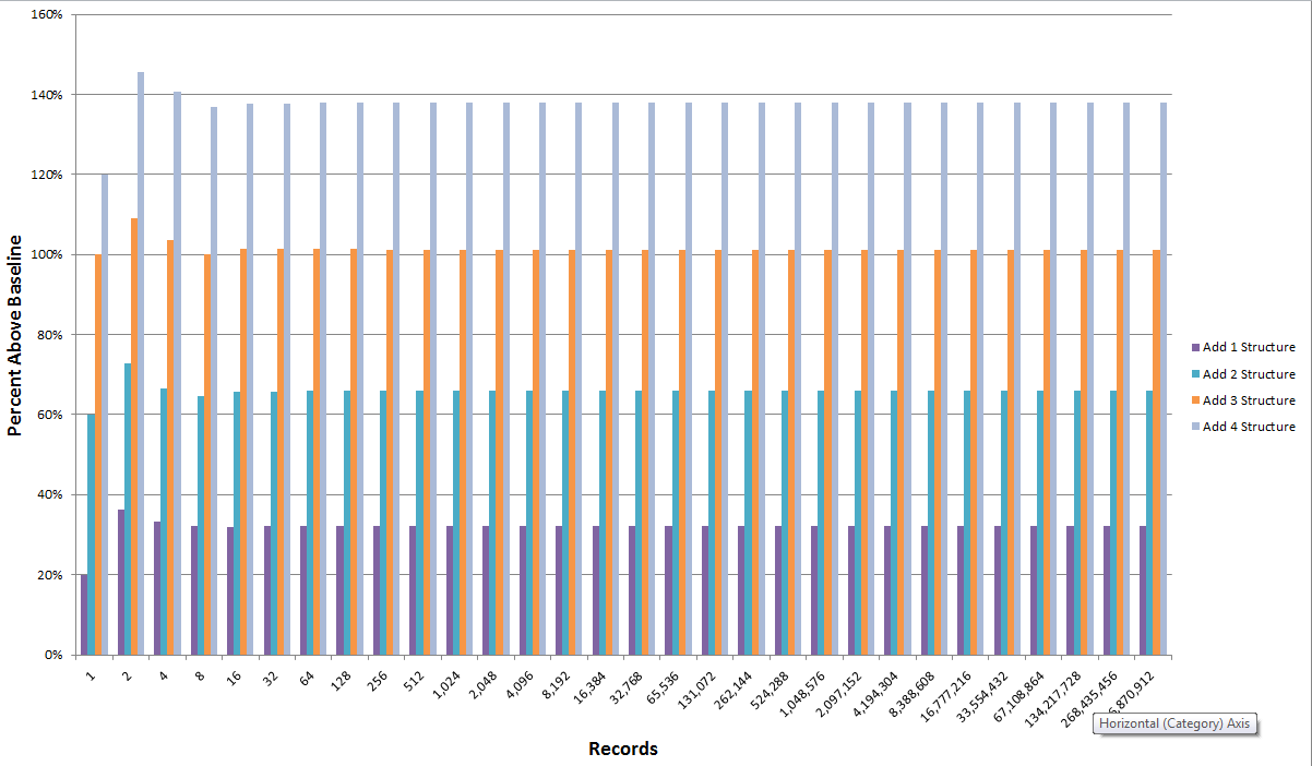
When we add structure across datasets the value improvements are a linear percent, as this figure shows:
For our Big Data example, each across-dataset structure characterization adds about 25% to 30% value per structure. Adding four structural characterizations, for example, more than doubles the “facts” assertion value (~ 140%) to the datasets.
Preview of Last Part
The last part forthcoming tomorrow will summarize the implications from the Viking algorithm on the role and importance of Big Structure to your organization’s Big Data efforts. Some caveats and future directions will conclude the series.


