Posted:August 19, 2020

Jump In! The Water is Fine
One of the reasons for finding a Python basis for managing our ontologies is to find a syntax that better straddles what the programming language requires with what the semantic vocabularies offer. In the last installment of this Cooking with Python and KBpedia series, we picked the owlready2 OWL management application in the hopes of moving toward that end. For the next lessons we will be trying to juggle new terminology and syntax from Python with the vocabulary and syntax of our KBpedia knowledge graphs. These terminologies are not equal, though we will try to show how they may correspond nicely with the use of the right mappings and constructs.

The first section of this installment is to present a mini-vocabulary of the terminology from KBpedia. Most of this terminology derives from the semantic technology standards of RDF, OWL and SKOS in which KBpedia and its knowledge graphs are written. Some of the terminology is unique to KBpedia. After this grounding we again load up the KBpedia graphs and begin to manipulate them with the basic CRUD (create-read-update-delete) actions. We will do that for KBpedia ‘classes’ in this installment. We will expand out to other major ontology components in later installments.

Basic KBpedia Terminology

In KBpedia there are three main groupings of constituents (or components). These are:

  • Instances (or individuals) — the basic, ‘ground level’ components of an ontology. An instance is an individual member of a class, also used synonymously with entity. The instances in KKO may include concrete objects such as people, animals, tables, automobiles, molecules, and planets, as well as abstract instances such as numbers and words. An instance is also known as an individual, with member and entity also used somewhat interchangeably. Most instances in KBpedia come from external sources, like Wikidata, that are mapped to the system;
  • Relations — a connection between any two objects, entities or types, or an internal attribute of that thing. Relations are known as ‘properties‘ in the OWL language;
  • Types (or classes or kinds) — are aggregations of entities or things with many shared attributes (though not necessarily the same values for those attributes) and that share a common essence, which is the defining determinant of the type. See further the description for the type-token distinction.

(You will note I often refer to ‘things’ because that is the highest-level (‘root’) construct in the OWL2 language. ‘Thing’ is also a convenient sloppy term to refer to everything in a given conversation.)

We can liken instances and types (or individual and classes, respectively, using semantic terminology) to the ‘nouns’ or ‘things’ of the system. Concepts are another included category. Because we use KBpedia as an upper ontology that provides reference points for aggregating external information, even things that might normally be considered as an ‘individual’, such as John F. Kennedy, are treated as a ‘class’ in our system. That does not mean that we are confusing John F. Kennedy with a group of people, just that external references may include many different types of information about ‘John F. Kennedy’ such as history, impressions by others, or articles referencing him, among many possibilities, that have a strong or exclusive relation to the individual we know as JFK. One reason we use the OWL2 language, among many, is that we can treat Kennedy as both an individual and an aggregage (class) when we define this entity as a ‘class’. How we then refer to JFK as we go forward — a ‘concept’ around the person or an individual with personal attributes — is interpreted based on context using this OWL2 ‘metamodeling’ construct. Indeed, this is how all of us tend to use natural language in any case.

We term these formal ‘nouns’ or subjects in KBpedia reference concepts. RefConcepts, or RCs, are a distinct subset of the more broadly understood ‘concept’ such as used in the SKOS RDFS controlled vocabulary or formal concept analysis or the very general or abstract concepts common to some upper ontologies. RefConcepts are selected for their use as concrete, subject-related or commonly used notions for describing tangible ideas and referents in human experience and language. RCs are classes, the members of which are nameable instances or named entities, which by definition are held as distinct from these concepts. The KKO knowledge graph is a coherently organized structure (or reference ‘backbone’) of these RefConcepts. There are more than 58,000 RCs in KBpedia.

The types in KBpedia, which are predominantly RCs but also may be other aggregates, may be organized in a hierarchical manner, which means we can have ‘types of types’. In the aggregate, then, we sometimes talk of these aggregations as, for example:

  • Attribute types — an aggregation (or class) of multiple attributes that have similar characteristics amongst themselves (for example, colors or ranks or metrics). As with other types, shared characteristics are subsumed over some essence(s) that give the type its unique character;
  • Datatypes — pre-defined ways that attribute values may be expressed, including various literals and strings (by language), URIs, Booleans, numbers, date-times, etc. See XSD (XML Schema Definition) for more information;
  • Relation types — an aggregation (or class) of multiple relations that have similar characteristics amongst themselves. As with other types, shared characteristics are subsumed over some essence(s) that give the type its unique character;
  • SuperTypes (also Super Types) — are a collection of (mostly) similar reference concepts. Most of the SuperType classes have been designed to be (mostly) disjoint from the other SuperType classes, these are termed ‘core’; other SuperTypes used mostly for organizational purposes are termed ‘extended’. There are about 80 SuperTypes in total, with 30 or so deemed as ‘core’. SuperTypes thus provide a higher-level of clustering and organization of reference concepts for use in user interfaces and for reasoning purposes; and
  • Typologies — flat, hierarchical taxonomies comprised of related entity types within the context of a given KBpedia SuperType (ST). Typologies have the most general types at the top of the hierarchy; the more specific at the bottom. Typologies are a critical connection point between the TBox (RCs) and ABox (instances), with each type in the typology providing a possible tie-in point to external content.

One simple organizing framework is to see a typology as a hierarchical organization of types. In the case of KBpedia, all of these types are reference concepts, some of which may be instances under the right context, organized under a single node or ‘root’, which is the SuperType.

As a different fundamental split, relations are the ‘verbs’ of the KBpedia system and cleave into three main branches:

  • Direct relations — interactions that may occur between two or more things or concepts; the relations are all extensional;
  • Attributes — the characteristics, qualities or descriptors that signify individual things, be they entities or concepts. Attributes are known through the terms of depth, comprehension, significance, meaning or connotation; that is, what is intensional to the thing. Key-value pairs match an attribute with a value; it may be an actual value, one of a set of values, or a descriptive label or string;
  • Annotations — a way to describe, label, or point to a given thing. Annotations are in relation to a given thing at hand and are not inheritable. Indexes or codes or pointers or indirect references to a given thing without a logical resolution (such as ‘see also’) are annotations, as well as statements about things, such as what is known as metadata. (Contrasted to an attribute, which is an individual characteristic intrinsic to a data object or instance, metadata is a description about that data, such as how or when created or by whom).

Annotations themselves have some important splits. One is the preferred label (or prefLabels), a readable string (name) for each of the RCs in KBpedia, and is the name most often used in user interfaces and such. altLabels are multiple alternate names for an RC, which when done fairly comprehensively are called semsets. A semset can often have many entries and phrases, and may include true synonyms, but also jargon, buzzwords, acronyms, epithets, slang, pejoratives, metonyms, stage names, diminuitives, pen names, derogatives, nicknames, hypochorisms, sobriquets, cognomens, abbreviations, or pseudonyms; in short, any term or phrase that can be a reference to a given thing.

These bolded terms have special meanings within KBpedia. To make these concepts computable, we also need correspondence to the various semantic language standards and then to constructs within Python and owlready2. Here is a high-level view of that correspondence:

KBpedia RDF/OWL (Protégé) Python + Owlready2
type Class A.
type of subClassOf A(B)
relation property
direct relation objectProperty i.R = j
datatypeProperty i.R.append(j)
annotation annotationProperty i.R.attr(j)
instance individual instance
instance i type A i = A()
isinstance(i,A)

The owlready2 documentation shows the breadth of coverage this API presently has to the OWL language. We will touch on many of these aspects in the next few installments. However, for now, let’s load KBpedia into owlready2.

Loading KBpedia

OK, so we are ready to load KBpedia. If you have not already done so, download and unzip this package (cwpk-18-zip from the KBpedia GitHub site. You will see two files named ‘kbpedia_reference_concepts’. One has an *.n3 extension for Notation3, a simple RDF notation. The other has an *.owl extension. This is the exact same ontology saved by Protégé in RDF/XML notation, and is the standard one used by owlready2. Thus, we want to use the kbpedia_reference_concepts.owl file.

Another reason we want to load this full KBpedia knowledge graph is to see if your current configuration has enough memory for the task. If, after the steps below, you are unable to load KBpedia, you may need a memory change to proceed. You may either need to change your internal memory allocations for Python or add more physical memory to your machine. We offer no further support, though outside research may help you diagnose and correct these conditions in order to proceed.

Relative addressing of files can be a problem in Python, since your launch directory is more often the current ‘root’ assumed. Launch directories move all over the place when interacting with Python programs across your system. A good practice is to be literal and absolute in your file addressing in Python scripts.

We are doing two things in the script below. The first is that we are setting the variable main to our absolute file address on our Window system. Note we could use the ‘r‘ (raw) switch to reference the Windows backslash in its file system syntax, r'C:\1-PythonProjects\kbpedia\sandbox\kbpedia_reference_concepts.owl'. We could also ‘escape’ the backward slash by preferencing each such illegal character with the ‘/’ forward slash. We can also rely on Python already accommodating Windows file notation.

The second part of the script below is to iterate over main and print to screen each line in the ontology file. This confirmation occurs when we shift+enter and the cell tells us the file reference is correct and working fine by writing the owl file to screen. BTW, if you want to get rid of the output file listing, you may use Cell → All Output → Clear to do so.

Which environment? The specific load routine you should choose below depends on whether you are using the online MyBinder service (the ‘raw’ version) or local files. See CWPK #17 for further details.
main = 'C:/1-PythonProjects/kbpedia/sandbox/kbpedia_reference_concepts.owl'   # note file change

with open(main) as fobj:                           
    for line in fobj:
        print (line)
import urllib.request 

main = 'https://raw.githubusercontent.com/Cognonto/CWPK/master/sandbox/builds/ontologies/kbpedia_reference_concepts.owl'
for line in urllib.request.urlopen(main):
    print(line.decode('utf-8'), end='')

Now that we know we successfully find the file at main, we can load it under the name of ‘onto’:

from owlready2 import *
onto = get_ontology(main).load()

Let’s now test to make sure that KBpedia has been loaded OK by asking the datastore what the base address is for the KBpedia knowledge graph:

print(onto.base_iri)
http://kbpedia.org/kbpedia/rc#

Great! Our knowledge graph is recognized by the system and is loaded into the local datastore.

In our next installment, we will begin poking around this owlready2 API and discover what kinds of things it can do for us.

NOTE: This article is part of the Cooking with Python and KBpedia series. See the CWPK listing for other articles in the series. KBpedia has its own Web site.
NOTE: This CWPK installment is available both as an online interactive file or as a direct download to use locally. Make sure and pick the correct installment number. For the online interactive option, pick the *.ipynb file. It may take a bit of time for the interactive option to load.
I am at best an amateur with Python. There are likely more efficient methods for coding these steps than what I provide. I encourage you to experiment — which is part of the fun of Python — and to notify me should you make improvements.

Posted by AI3's author, Mike Bergman Posted on August 19, 2020 at 10:51 am in CWPK, KBpedia, Semantic Web Tools | Comments (2)
The URI link reference to this post is: https://www.mkbergman.com/2348/cwpk-18-basic-terminology-and-load-kbpedia/
The URI to trackback this post is: https://www.mkbergman.com/2348/cwpk-18-basic-terminology-and-load-kbpedia/trackback/
Posted:August 18, 2020

owlready2 Appears to be a Capable Option

In the CWPK #2 and #4 installments to this Cooking with Python and KBpedia series, we noted that we would reach a decision point when we needed to determine how we will manipulate our knowledge graphs (ontologies) using the Python language. We have now reached that point. Our basic Python environment is set (at least in an initial specification) and we need to begin inputting and accessing KBpedia to develop and test our needed management and build functions.

In our own efforts over the past five years or more, we have used the Java OWL API initially developed by the University of Manchester. The OWL API is an integral part of the Protégé IDE (see CWPK #5) and supports OWL2. The API is actively maintained. We have been very pleased with the API’s performance and stability in our earlier KBpedia (and other ontology) efforts. In our own Clojure-based work we have used a wrapper around the OWL API. A wrapper using Python is certainly a viable (perhaps even best) approach to our current project.

We still may return to this approach for reasons of performance or capabilities, but I decided to first explore a more direct approach using a Python language option. This decision is in keeping with this series’ Python education objectives. I prefer for these lessons to use a consistent Python style and naming conventions, rather than those in Java. I was also curious to evaluate and test what presently exists in the marketplace. We may gain some advantages from a more direct approach; we may also discover some gotchas or deadends that initial due diligence missed. We can always return to Plan B with a wrapper around the existing OWL API.

If we do need to revert and take the wrapper approach, the leading candidate for the wrapper is py4j. Initial research suggests other Python bridges to Java such as Jython or JPype are less efficient and less popular than py4j. pyJNIus had a similar objective to py4j but has seen no development activity for 4-6 years. The ROBOT tool for biomedical ontologies points the way to how Python can link through py4j. Even if our Python-based approach herein works great, we still may want to embrace py4j as we move forward given the wealth of ontology-related applications written in Java. But I digress.

There is no acclaimed direct competitor to the OWL API in Python, though there are pieces that may approximate its capabilities. Frankly, I was surprised after beginning my due diligence with the relative dearth of Python tools for working with OWL. Many of the Python projects that do or did exist harken back years. There was a bulge of tool-making in the mid-2000s using Python that has since cooled substantially, with two notable exceptions I discuss below.

One of those exceptions is RDFLib, a Python library for working with RDF. RDFLib provides a useful set of parsers and serializers and a plug-in architecture, but directly lacks OWL 2 support. FuXi was an OWL reasoner based on RDFLib that used a subset of OWL, but is now abandoned. SuRF is an object-RDF mapper based on RDFlib that enables manipulations of RDF triples, but is somewhat dated. rdftools had a similar objective to RDFLib, but has been abandoned from about 5-7 yrs ago. owlib is a 5-yr old API to OWL built using RDFLib to simplify working with OWL constructs; it has not been updated and is inactive. More currently, infixowl is a RDFLib Python binding for the OWL abstract syntax, which makes it more like the wrapper alternative. Though not immediately applicable to our OWL needs, we may later embrace RDFLib for parsers and serializers or as a useful library for the typologies in KBpedia.

Then there are a number of tools independent of RDFLib. SETH was an attempt at a Python OWL API that still required the JVM from about a dozen years back, and is now largely abandoned (though available via CVS repository). funowl is a pythonic API that follows the OWL functional model for constructing OWL and it provides a py4j or equivalent wrapper to the standard Java OWL libraries. It appears to be active and is worth keeping an eye on. The ontobio Python module is a library for working with ontologies and associations to outside entities, though it is not an ontology manager.

Fortunately, the second exception is owlready2, a module for ontology-oriented programming in Python 3, including an optimized RDF quadstore. A number of things impressed me about owlready2 in my due diligence. First, its functionality fit the bill for what I wanted to see in an ontology manager dealing with all CRUD (create-read-update-delete) aspects of an ontology and its components. Second, I liked the intent and philosophy behind the system as expressed in its original academic paper and home Web site (see Additional Documentation below). Third, the project is being actively maintained with many releases over the past two years. Fourth, the documentation level was comparatively high for an open-source project and clearly written and understandable. And, last, there is an existing extension to owlready2 that adds support for RDFLib, should we also decide to add that route.

One concern arising from my diligence is the lack of direct Notation3 (N3) file support in owlready2, since all of KBpedia’s current ontology files are in N3. According to owlready2’s developer, Jean-Baptiste Lamy, N-Triples, which are a subset of N3, are presently supported by owlready2. We can test and see if our N3 constructs load or not. If they do not, we can save out our ontology files in RDF/XML, which owlready2 does support. (Indeed, use of the RDF/XML format has proven to be the better approach.) Alternatively, we can do file conversions with RDFLib or the Java OWL API. File format conversions and compatibility will be a constant theme in our work, and this potential hurdle is not unlike others we may face.

Thus, while the pickings were surprisingly thin for off-the-shelf OWL tools in Python, owlready2 appears to have the requisite functionality and currentness and to be a reasonable initial choice. Should this choice prove frustrating, we will likely fall back onto the py4j wrapper to the OWL API or funowl.

So, now with the choice made, it is time to set up our directory structure and install owlready2.

Here is our standard main directory structure with the owlready2 additions noted:

|-- PythonProject                                             
|-- Python
|-- [Anaconda3 distribution]
|-- Notebooks
|-- CWPKNotebook
|-- owlready2 # place it at top level of project
|-- kg # for knowledge graphs (kgs) and ontologies
|-- scripts # for related Python scripts
|-- TBA

After making these changes on disk, it is time to install owlready2, which is easy:

    conda install -c conda-forge owlready2

You will see the reports to the screen terminal as we noted before, and you will need to agree to proceed. Assuming no errors are encountered, you will be returned to the command window prompt. You can then invoke ‘Jupyter Notebook‘ again.

Finding and Opening Files

Let’s begin working with owlready2 by loading and reading an ontology/knowledge graph file. Let’s start with the smallest of our KBpedia ontology files, kko.owl (per the instructions above this is the kko.n3 file converted to RDF/XML in Protégé). (You may download this converted file from here.) I will also assume you stored this file under the owlready2/kg directory noted above.

Important Note: You may be working with these interactive notebooks either online with MyBinder or from your own local file system. In the first case, the files you will be using will be downloaded from GitHub; in the second case, you will be reading directly from your local directory structure. In the instructions below, and in ALL cases where external files are used, we will show you the different Python commands associated with each of these options.

As you begin to work with files in Python on Windows, here are some initial considerations:

  • In Windows, a full file directory path starts with a drive letter (C:, D:. etc.). In Linux and OS-X, it starts with “/
  • Python lets you use OS-X/Linux style slashes “/” in Windows. Recommended is to use a format such as ‘C:/Main/FirstDirectory/second-directory/my-file.txt
  • Relative addressing is allowed, with the current directory understood to be the one where you started your interpreter (Jupyter Notebook in our case). However, that is generally not best practice. Python embraces the concept of Current Working Directory. CWD is the folder your Python is operating from, which might vary by application, such as Jupyter Notebook. The CWD is the 'root‘ for your current session. What this means is that relative file addresses can be tricky to use. You are best off using the absolute reference to all of your files.

When you work with online file documents, you will need to use different Python commands and conventions, as the examples below show. We will offer more explanation on this specific option when the code below is presented.

Here are some general references that can explain files and paths further:

To find what your CWD is for your current session:

import os
dir(os)

Note there are a couple of things going on in this snippet. First, we have imported the Python built-in module called ‘os‘. Not all commands are brought into memory when you first invoke Python. In this case, we are invoking (or ‘importing’) the os module.

Second, we have invoked the dir command to get a listing of the various functions within the os module. So, go ahead and shift+enter this cell or Run it from the Jupyter Notebook menu to see what os contains.

We can invoke other functions with a similar syntax. Another option besides dir is to get help on the current module:

help(os)

Note these same dir and help commands can be applied to any (module) active in the system.

This next example shows another function in os called ‘walk‘. We invoke this function by calling the combined module and function notation using the dot (.) syntax (‘os.walk‘). We will add a couple more statements to get our directory listing to display (‘print()‘) the directory file names to screen:

for dirpath, dirnames, files in os.walk('.'):
    print(f'Found directory: {dirpath}')
    for file_name in files:
        print(file_name)

One of the first things you will learn about Python is that there are often multiple modules, and modules within external libraries, that may be invoked for a given task. It takes time to discover and learn these options, but that is also one of the fun parts of the language.

Our next example shows just this, using a new package, pathlib, useful for local files, that has some great path management functions. (This library will be one of our stalwarts moving forward.)

Remember we can import functions from add-ons beyond the Python built-ins. We do so via modules again using the import statement, but we now need to identify the library (or ‘package’) where that module resides. We do so via the ‘from‘ statement. Remember, external libraries need to be downloaded and registered via Anaconda (conda or conda-forge) prior to use if they are not already installed on your system. (Recall that our installed packages are at C:\1-PythonProjects\Python\pkgs based on my own configuration.

In this next example we are using the home command within the Path module in the pathlib package. The home command tells us where the ‘root‘ is for our current notebook:

from pathlib import Path
home = Path.home()
print(home)
C:\Users\Michael

Windows is a tricky environment for handling file names, since the native operating system (OS) requires back-clashes (‘\‘) rather than forward-slashes (‘/‘) and also requires the drive designation for absolute paths. We also have the issue of relative paths, which because of CWD (common working directory) can get confused in Python (or rather, in our use of Python).

One habit is to adopt the convention of declaring your file targets as a variable (say, ‘path‘), make sure the reference is good, and then refer to the ‘path‘ object in the rest of the code to prevent confusion. One code approach to this, including a print of the referenced file is:

path = r'C:\1-PythonProjects\owlready2\kg\kko.owl'         # see (A)
# path = 'https://raw.githubusercontent.com/Cognonto/CWPK/master/sandbox/builds/ontologies/kko.owl'      # see (A)
with open(path) as fobj:                                   # see (B)
    for line in fobj:
        print (line, end='')

Note, this example may not work unless you are using local files.

We get the absolute file name (A) on Windows by going to its location within Windows Explorer, highlighting our desired file in the right panel, and then right-clicking on the path listing shown above the pane and choosing ‘Copy address as text’; that is the information placed between the quotes on (A). Note also the ‘r‘ switch on this line (A) (no space after ‘r‘!), which means ‘raw’ and enables the Windows backslashes to be interpreted properly. Go ahead and shift+enter this file and see the listing (which is also useful to surface any encoding issues, which will appear at the end of the file listing should they exist).

Now, the example above is for local files. If you are using the system via MyBinder, we need to load and view our files from online. Here is a different format for accessing such information:

import urllib.request 

path = 'https://raw.githubusercontent.com/Cognonto/CWPK/master/sandbox/builds/ontologies/kko.owl'
for line in urllib.request.urlopen(path):
    print(line.decode('utf-8'), end='')

A couple of items for this format deserve comment. First, we need to import a new package, urllib, that carries with it the functions and commands necessary for accessing URLs. There are multiple options available in Python for doing so. This particular one presents, IMO, one of the better formats for viewing text files. Second, we declare the UTF-8 encoding, a constant requirement and theme through the rest of this CWPK series. And, third, we add the attribute option of end='' in our print statement to eliminate the extra lines in the printout that occur without it. Python functions often have many similar options or switches available.

In any case, the above gives us the basis to load the upper ontology of KBpedia called KKO. We now turn to how we begin to manage our knowledge graphs.

Import an Ontology

So, let’s load our first ontology into owlready2 applying some of these concepts:

from owlready2 import *
# the local file option
# onto = get_ontology(path).load()

# the remote file (URL) option
onto = get_ontology(path).load()

Inspect Ontology Contents

We do not get a confirmation that the file loaded OK, the object name of which is onto, except no error messages appeared (which is good!). Just to test if everything proceeded OK, let’s ask the system to return (print to screen) a known class from our kko.owl ontology called ‘Generals‘:.

print(onto.Generals)
        

Can apply to all of the ontology components (in this case the class, ‘Generals’).

We can also list all of the classes in the ontology:

list(onto.classes())
list(onto.disjoint_classes())

Armed with these basics we can begin to manipulate the components in our knowleldge graph, the topic for our next installment.

Additional Documentation

Here is additional documentation on owlready2:

NOTE: This article is part of the Cooking with Python and KBpedia series. See the CWPK listing for other articles in the series. KBpedia has its own Web site.
NOTE: This CWPK installment is available both as an online interactive file or as a direct download to use locally. Make sure and pick the correct installment number. For the online interactive option, pick the *.ipynb file. It may take a bit of time for the interactive option to load.
I am at best an amateur with Python. There are likely more efficient methods for coding these steps than what I provide. I encourage you to experiment — which is part of the fun of Python — and to notify me should you make improvements.

Posted by AI3's author, Mike Bergman Posted on August 18, 2020 at 9:40 am in CWPK, KBpedia, Semantic Web Tools | Comments (4)
The URI link reference to this post is: https://www.mkbergman.com/2347/cwpk-17-choosing-and-installing-an-owl-api/
The URI to trackback this post is: https://www.mkbergman.com/2347/cwpk-17-choosing-and-installing-an-owl-api/trackback/
Posted:August 17, 2020

Most of the Effort in Coding is in the Planning

With the environment in place, it is now time to plan the project underlying this Cooking with Python and KBpedia series. This installment formally begins Part II in our CWPK installments.

Recall from the outset that our major objectives of this initiative, besides learning Python and gaining scripts, were to manage and exploit the KBpedia knowledge graph, to expose its build and test procedures so that extensions or modifications to the baseline KBpedia may be possible by others, and to apply KBpedia to contemporary challenges in machine learning, artificial intelligence, and data interoperability. These broad objectives help to provide the organizational backbone to our plan.

We can thus see three main parts to our project. The first part deals with managing, querying, and using KBpedia as distributed. The second part emphasizes the logical build and testing regimes for the graph and how those may be applied to extensions or modifications. The last part covers a variety of advanced applications of KBpedia or its progeny. As we define the tasks in these parts of the plan, we will also identify possible gaps in our current environment that we will need to rectify for progress to continue. Some of these gaps we can identify now and so filling them will be some of our most immediate tasks. Other gaps may only arise as we work through subsequent steps. In those instances we will need to fill the gaps as encountered. Lastly, in terms of scope, while our last part deals with advanced applications that we can term ‘complete’ at some arbitrary number of applications, the truth is that applications are open-ended. We may continue to add to the roster of advanced applications as time and need allows.

Important Series Note: As first noted in CWPK #14, this current installment marks the first that every new CWPK article is now available as an interactive Jupyter Notebook page. The first interactive installment was actually CWPK #14, and we have reached back and made those earlier pages available as well.

Each of these new CWPK installments is available both as an online interactive file or as a direct download to use locally. For the online interactive option, pick one of the *.ipynb files. The MyBinder service we are using for the online interactive version maintains a Docker image for each project. Depending on how long it has been since someone last requested a CWPK interactive page, sometimes access may be rapid since the image is in cache, or it may take a bit of time to generate another image anew. We discuss this service more in CWPK #57.

Part I: Using and Managing KBpedia

Two immediate implications of the project plan arise as we begin to think it through. First, because of our learning and tech transfer objectives for the series, we have the opportunity to rely on the electronic notebook aspects of Jupyter to deliver on these objectives. We thus need to better understand how to mix narrative, working code, and interactivity in our Jupyter Notebook pages. Second, since we need to bridge between Python programs and a knowledge graph written in OWL, we will need some form of application programming interface (API) or bridge between these programmatic and semantic worlds. It, too, is a piece that needs to be put in place at the outset.

This additional foundation then enables us to tackle key use and management aspects for the KBpedia knowledge graph. First among these tasks are the so-called CRUD (create-read-update-delete) activities for the structural components of a knowledge graph:

  • Add/delete/modify classes (concepts)
  • Add/delete/modify individuals (instances)
  • Add/delete/modify object properties
  • Add/delete/modify data properties and values
  • Add/delete/modify annotations.

We also need to expand upon these basic management functions in areas such as:

  • Advanced class specifications
  • Advanced property specifications
  • Multi-lingual annotations
  • Load/save of ontologies (knowledge graphs)
  • Copy/rename ontologies.

We also need to put in place means for querying KBpedia and using the SPARQL query language. We can enhance these basics with a rules language, SWRL. Because our use of the knowledge graph involves feeding inputs to third-party machine learners and natural language processors, we need to add scripts for writing outputs to file in various formats. We want to add to this listing some best practices and how we can package our scripts into reusable files and libraries.

Part II: Building, Testing, and Extending the Knowledge Graph

Though KBpedia is certainly usable ‘as is’ for many tasks, importantly including as a common reference nexus for interoperating disparate data, maximum advantage arises when the knowledge graph encompasses the domain problem at hand. KBpedia is an excellent starting point for building such domain ontologies. By definition, the scope, breadth, and depth of a domain knowledge graph will differ from what is already in KBpedia. Some existing areas of KBpedia are likely not needed, others are missing, and connections and entity coverage will differ as well. This part of the project deals with building and logically testing the domain knowledge graph that morphs from the KBpedia starting point.

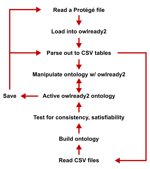
For years now we have built KBpedia from scratch based on a suite of canonically formatted CSV input files. These input files are written in a common UTF-8 encoding and duplicate the kind of tuples found in an N3 (Notation3) RDF/OWL file. As a build progresses through its steps, various consistency and logical tests are applied to ensure the coherence of the built graph. Builds that fail these tests are error flagged, which requires fixes to the input files, before the build can resume and progress to completion. The knowledge graph that passes these logical tests might be used or altered by third-party tools, prominently including Protégé, during the use of and interaction with the graph. We thus also need methods for extracting out the build files from an existing knowledge graph in order to feed the build process anew. These various workflows between graph and build scripts and tools is shown by Figure 1:

General Workflow of the KBpedia Project
Figure 1: General Workflow of the KBpedia Project

This part of the plan will address all steps in this workflow. The use of CSV flat files as the canonical transfer form between the applications also means we need to have syntax and encoding checks in the process. Many of the instructions in this part deal with good practices for debugging and fixing inconsistent or unsatisfied graphs. At least as we have managed KBpedia to date, every new coherent release requires multiple build iterations until the errors are found and corrected. (This area has potential for more automation.)

We will also spend time on the modular design of the KBpedia knowledge graph and the role of (potentially disjoint) typologies to organize and manage the entities represented by the graph. Here, too, we may want to modify individual typologies or add or delete entire ones in transitioning the baseline KBpedia to a responsive domain graph. We thus provide additional installments focused solely on typology construction, modification, and extension. Use and mapping of external sources is essential in this process, but is never cookie-cutter in nature. Having some general scripts available plus knowledge of creating new relevant Python scripts is most helpful to accommodate the diversity found in the wild. Fortunately, we have existing Clojure code for most of these components so that our planning efforts amount more to a refactoring of an existing code base into another language. Hopefully, we will also be able to improve a bit on these existing scripts.

Part III: Advanced Applications

Having full control of the knowledge graph, plus a working toolchest of applications and scripts, is a firm basis to use the now-tailored knowledge graph for machine learning and other advanced applications. The plan here is less clear than the prior two parts, though we have documented existing use cases with code to draw upon. Major installments in this part are likely in creating machine learning training sets, in creating corpora for unsupervised training, generating various types (word, statement, graph) of embedding models, selecting and generating sub-graphs, mapping external vocabularies, categorization, and natural language processing.

Lastly, we reserve a task in this plan for setting up the knowledge graph on a remote server and creating access endpoints. This task is likely to occur at the transition between Parts II and III, though it may prove opportune to do it at other steps along the way.

NOTE: This article is part of the Cooking with Python and KBpedia series. See the CWPK listing for other articles in the series. KBpedia has its own Web site.
NOTE: This CWPK installment is available both as an online interactive file or as a direct download to use locally. Make sure and pick the correct installment number. For the online interactive option, pick the *.ipynb file. It may take a bit of time for the interactive option to load.
I am at best an amateur with Python. There are likely more efficient methods for coding these steps than what I provide. I encourage you to experiment — which is part of the fun of Python — and to notify me should you make improvements.

Posted by AI3's author, Mike Bergman Posted on August 17, 2020 at 10:01 am in CWPK, KBpedia, Semantic Web Tools | Comments (0)
The URI link reference to this post is: https://www.mkbergman.com/2345/cwpk-16-planning-the-project/
The URI to trackback this post is: https://www.mkbergman.com/2345/cwpk-16-planning-the-project/trackback/
Posted:August 14, 2020

Recipes for Jupyter Notebooks Going Forward

In the last installment of the Cooking with Python and KBpedia series, we began to learn about weaving code and narrative in a Jupyter Notebook page. We also saw that we can generate narratives to accompany our code with the Markdown mark-up language, though it is not designed (in my view) for efficient document creation. Short explanations between code snippets are fine in Jupyter Notebook, but longer narratives or ones where formatting or decorating are required are fairly difficult. (For an update, see the NB box at the conclusion of this installment.) Further, we also want to publish Web pages independent of our environment. What I describe in this CWPK installment is how I combine standard Web page editing and publishing with Jupyter, as well as the starting parts to my standard workflow.

Having a repeatable and fairly efficient workflow for formulating a lesson or question, then scoping it out framed with introduction and working parts, and then skeletonizing it such that good working templates can be put in place is important when one contemplates progressing through all of the stages of discovering, addressing, and documenting a project. In the case of this CWPK series, this is not a trifling consideration. I am anticipating literally dozens of installments in this series; heck, we are already at installment #15 and we haven’t begun yet to code anything in Python! We could stitch together more direct methods of doing a given task, but that will not necessarily arm us to do a broader set of tasks.

Not everyone prefers my style of trying to get systems and game plan in place before tackling a big task, in which case I suggest you skip to the end where we conclude with a discussion of directory organization. For this initial part, however, I will assume that you want to sometimes rely on an interacting coding environment and other times want to generate narratives efficiently. In this use case, the ability to ‘round-trip‘ between HTML editing and Jupyter is an important consideration. Efficiency and document size are relevant considerations, too.

Recall in our last installment that we pointed to two ways to get HTML pages from a Jupyter Notebook: 1) either from a download, or 2) from invoking the nbconvert service from a command window. We could not invoke nbconvert from within a notebook page because it is a Jupyter service. This next frame shows the file created from the article herein using the download method. You invoke the cell by entering shift+enter to call up the file, and then, once inspected, use Cell → All Output → Clear to clear and collapse the view area:

with open('files/cwpk-15-using-notebooks-download.txt', 'r') as f:
    print(f.read())

I should mention that both the nbconvert and download methods produce similarly bloated files. Go ahead, scroll through it. While the generated file renders very well, it is about 10x larger than the original HTML file that captures its narrative (13,644 v 397 lines; 298 K v 30 K). This bloat in file size is due to the fact that all of the style information (*.css) contained in the original document gets re-expressed in this version, along with much other styling information not directly related to this page. Thus, while the generation of the page is super easy, and renders beautifully, it is an overweight pig. We could spend some time whittling down this monster to size with some of the built-in functionality of nbconvert, but why not deal that problem using Pandoc directly upon which nbconvert is based?

So, in testing the cycle from HTML to notebooks and back again, we find that certain aspects of generating project documentation present challenges. In working through the documentation for this series I have found these types of problem areas for round-tripping:

  • Use of a standard, formatted header (with logo)
  • Use of standard footers (notification boxes in our case)
  • Centering images
  • Centering text
  • Tables, and
  • Loss of the interactive functionality in the notebook in the HTML.

Only the last consideration is essential to create useful project and code documentation. However, if one likes professional, well-formatted pages with loads of images and other pretty aspects, it is worth some time to work out productive ways to handle these aspects. In broad terms, for me, that means to be able to move between Web page authoring and interactive code development, testing, and documentation. I also decided to devote some time to these questions as a way to better understand the flexibilities and power of the tools we have chosen. We will always encounter gaps in knowledge when working new problems. I’d like to find the practical balance between the de minimus path to get something done with learning enough to be able to travel similar paths in the future, perhaps even in a production mode.

Since Markdown is a superset of HTML it is not possible to round-trip using Markdown alone within Jupyter Notebook. Fortunately, many Markdown interpreters, including Jupyter, accept some limited HTML in documents. There are two ways that may happen. The first is to use one of the so-called ‘magic’ terms in iPython, the command shell underneath Jupyter Notebook. By placing the magic term %%html at the start of a notebook Markdown cell, we instruct the system to render that entire cell as HTML. Since it is easy to stop a cell and add a new one below it, we can ‘fence’ such aspects easily in our notebook code bases. I encourage you to study other ‘magic’ terms from the prior link that are shortcuts to some desired notebook capabilities.

A second way to use HTML in notebooks is to embed HTML tags. This way is trickier since the various Markdown evaluation engines — due to Markdown’s diversity of implementations — may recognize different tags or, when recognized, treat them differently. One of the reasons to embrace Pandoc, introduced in the last installment, is to accept its standard way of handling languages, markups, formats, and functions.

Boiled down to its essence, then, we have two functional challenges in round-tripping:

  1. Loss of HTML tags and styling with Markdown
  2. Loss of notebook functionality in HTML.

One of Pandoc’s attractions is that both <div> and <span> can be flagged to be skipped in the conversions, which means we can isolate our HTML changes to these tag types, with divs giving us block ‘fencing’ capabilities and spans inline ‘fencing’ capabilities. (There are also Lua filter capabilities with Pandoc to provide essentially unlimited control over conversions, but we will leave that complexity outside of our scope.) Another observation we make is that many of the difficult tags that do not round-trip well deal with styling or HTML tags that can be captured via CSS styling.

Another challenge that must be deciphered are the many flavors of Markdown that appear in the wild. Pandoc handles many flavors of Markdown, including the specified readers of markdown, markdown_strict, markdown_mmd, markdown_phpextra, and gfm (GitHub-flavored Markdown). One can actually ingest any of these flavors in Pandoc and express any of the others. As I noted in the last installment, Pandoc presently has 33 different format readers from Word docs to rich text and can write out nearly twice that many in different formats. For our purposes, however, it is best to choose Pandoc’s canonical internal form of markdown. However, besides translation purposes, the gfm option likely has the broadest external applicability.

OK, so it appears that Pandoc’s own flavor of Markdown is the best conversion target and that we will try to move problem transfer areas to div and span. As for the loss of notebook functionality in HTML, there is no direct answer. However, because an interactive notebook page is organized in a sequence of cells, we can segregate activity areas from interactive areas in our documents. That does not give us complete document convertibility, but we can do it in sections if need be after initial drafting. With this basic approach decided, we begin to work through the issues.

After testing inline styling, we see that we can find recipes that move the CSS and related HTML (such as <center> or <i> or <italics>) between our HTML and notebook environments without loss. Once we go beyond proofs of concept, however, we want to be able to capture our CSS information in styling class and ID designations so that we not need to duplicate lengthy styling code. However, handling and referencing CSS stylesheets is not straightforward with the complexity of applications and configuration files of an Anaconda Python distribution and environment. For a very useful discussion of CSS in this context see Jack Northrup’s notebook on customizing CSS.

Now, the tools at both ends of this process, Jupyter Notebook and Pandoc, both recognize users will want their own custom.css files to guide these matters. But, of course, each tool has a different location and mechanism for specifying this. There is surprisingly little documentation or guidance on the Web for how to handle these things. Most of the references I encountered on these matters were incorrect. We have two fundamental challenges in this quest: 1) how do we define and where do we locate our custom.css file on disk?; and 2) what are our command-line instructions to best guide the two round-trip conversion steps? We will use Pandoc and proper stylesheet locations to guide both questions.

Let’s take the first trip of moving from HTML draft into an operating shell for Jupyter Notebook. First, as we draft material with an HTML editor, we are going to want to store our custom.css information that we need to segregate into some pre-defined, understood location. One way to do that is through a relative location in relation to where our authored HTML document resides. An easy choice is to create a sub-directory of files that is placed immediately below where our HTML document resides. If we follow this location, we may always find the stylesheet (CSS) in the relative location of ‘files/custom.css‘. (You may name the subdirectory something different, but it is probably best to retain the name of ‘custom.css‘ since that is expected by Jupyter.) However, those same CSS specifications need to be available to Jupyter Notebook, which follows different file look-up conventions. One way to discover where Jupyter Notebook expects to find its supplementary CSS files is to open the relevant notebook page and save it as HTML (download or nbconvert or Pandoc methods). When you open the HTML file with an editor, look for the reference to ‘custom.css‘. That will give you the file location in relation to your document’s root. In my case, this location is C:\1-PythonProjects\Python\Lib\site-packages\notebook\static\custom. For your own circumstance, it may also be under the \user\user\ profile area depending on whether you first installed Anaconda for an individual user. At any rate, look for the \Lib\ directory and then follow the directory cascade under your main Python location.

NB: Unfortunately, should you later update your Jupyter Notebook package, you may find that your custom.css is overwritten with the standard, blank placeholder. You may again need to copy your active version into this location.

Once you have your desired CSS both where Pandoc will look for it (again, relative is best) and where Jupyter Notebook will separately look for it, we can concentrate on getting our additional styles into custom.css, which you may click on to see its contents for this current page. Once we have populated custom.css, it is now time to figure out the conversion parameters. There is much flexibility in Pandoc for all aspects of instructing the application at the command line. I present one hard-earned configuration below, but for your own purposes, I strongly recommend you inspect the PDF version of the Pandoc User Guide should you want to pursue your own modifications. At any rate, here is the basic HTML → Notebook initial conversion, using this current page as the example:

$ pandoc -f html -t ipynb+native_divs cwpk-15-using-notebooks.html -o cwpk-15-using-notebooks.ipynb

Here is what these command-line options and switches mean:

  • -f html-f (also --from) is the source or from switch, with html indicating the source format type. Multiple types are possible, but only one may be specified at a time
  • -t ipynb-t (also --to) is the target of the conversion, with ipynb in this case indicating a notebook document. Multiple types are possible, but only one may be specificed here
  • +native_divs – this is a conversion switch that tells Pandoc to retain the content within a native HTML div in the source
  • cwpk-15-using-notebooks.html – this is the source file specification. There are defaults within Pandoc that allow -f html to not be specified, for example and for other formats, once this input file type is specified
  • -o cwpk-15-using-notebooks.ipynb – this is the output (-o) file name; if left unspecified, the default is to write the original file name with the new .ipynb extension (or whatever target format was specified).

These commands and switches require the Windows command window or PowerShell to be opened in the same directory as the *.html document you are converting when you instruct at the command line. Upon entering this command, the appearance of the prompt tells you the conversion proceeded to completion.

This command will now establish a new notebook file (*.ipynb) in the same directory. Please make sure this directory location is under the root you established when you installed Jupyter Notebook (see CWPK #10 if you need to refresh that or change locations).

When you invoke Jupyter Notebook and call up the new *.ipynb file, it will open as a single Markdown cell. If you need to split that input into multiple parts in order to interweave interactive parts, double-click to edit, cut the sections you need to move, Run the cell, add a cell below, and paste the split section into the new cell. In this way, you can skeletonize your active portions with existing narrative.

Upon completing your activities and additions and code tests within Notebook, you may now save out your results to HTML for publishing elsewhere. Again, you could Download or use nbconvert, but to keep our file sizes manageable and to give ourselves the requisite control we will again do this conversion with Pandoc. After saving your work and exiting to the command window, and while still in the current working directory where the *.ipynb resides, go ahead and issue this command at the command window prompt:

$ pandoc -s -f ipynb -t html -c files/custom.css --highlight-style=kate cwpk-15-using-notebooks.ipynb -o cwpk-15-using-notebooks-test.html

There we have it! We now have our recipes to move from HTML to *.ipynb and the reverse!

Here is what the new command-line options and switches mean:

We have now reversed the -f and -t switches since we are now exporting as HTML; again, multiple format options may be substituted here (though specific options may change depending on format)

  • -s means to process the export as standalone, which will bring in the HTML information outside of the <body> tags
  • -c (or --css=) tells the writer where to find the supplementary, external CSS file. This example is the files subdirectory under the current notebook; the file could be whatever.css, but we keep the custom.css name to be consistent with the required name for Jupyter (even though in a different location)
  • --highlight-style=kate is one of the language syntax highlighting options available in Pandoc; there are many others available and you may also create your own
  • -o cwpk-15-using-notebooks-test.html – is an optional output only if we want to change the base name from the input name; during drafting it is recommended to use another name (-test) to prevent inadvertent overwriting of good files.

Upon executing this command, you will get a successful export, but a message indicating you did not provide a title for the project and it will default to the file name as shown by Figure 1:

Message at HTML Export
Figure 1: Message at HTML Export

There are metadata options you may assign at the command line, plus, of course, many other configuration options. Again, the best consolidated source for learning about these options is in the PDF Pandoc Users Guide. This document is kept current with the many revisions that occur frequently for Pandoc.

The next panel shows the HTML generated by this export. Note this document is much smaller (10x) than the version that comes from the download or nbconvert methods:

with open('files/cwpk-15-using-notebooks-html.txt', 'r') as f:
    print(f.read())

This HTML export is good for publication purposes, but lacks the interactivity of its interactive parent. You should thus refrain from such exports until development is largely complete. In any case, we still see static sections for the interactive portions of the notebook. These were styled according to custom.css.

NB: The Web pages that appear on my AI3 blog are the HTML conversions of these interactive notebook pages. The information box at the bottom of each installment page instructs as to where you may obtain the fully interactive versions.

Using similar commands you can also produce outputs in other formats, such as this one for the GitHub flavor of Markdown using this command line instruction:

$ pandoc -s -f ipynb -t gfm -c files/custom.css --highlight-style=kate cwpk-15-using-notebooks.ipynb

Note we have changed the -t to option to gfm and have removed the -o output option because we will use the same notebook file name. Here is the output from that conversion:

with open('files/cwpk-15-using-notebooks-md.txt', 'r') as f:
    print(f.read())

You can see that headers are more cleanly shown by # symbols, and that gfm is a generally clean design. It is becoming the de facto standard for shared Markdown.

Of course, no export is necessary for the actual notebook file since they are plain text. As noted in earlier installments, Jupyter Notebook files are natively expressed in JavaScript Object Notation (JSON). This is the only file representation that contains transferrable instructions for the interactive code cells in the notebook page. This JSON file is for the same content expressed in the files above:

with open('files/cwpk-15-using-notebooks-ipynb.txt', 'r') as f:
    print(f.read())

Mastery of these tools is a career in itself. I’m sure there are better ways to write these commands or even how to approach the workflow. As the examples presently stand there are a few minor glitches, for example, that keep this round-tripping from being completely automatic. Relative file locations get re-written with an ‘attachment:‘ prefix during the round-trip, which must be removed from the HTML code to get images to display. For some strange reason, images also need to have a width entry (e.g., width="800") in order not to be converted to Markdown format. Also, in some instances HTML code within a div gets converted to Markdown syntax, which then can not be recognized when later writing to HTML. The Pandoc system is full-featured and difficult to master without, I am sure, much use.

In working with these tools, here is what I have discovered to be a good starting workflow:

  1. Author initial skeleton in HTML. Write intro, get references and links, set footer. Try to use familiar editing tools to apply desired formatting and styles
  2. Add blocks and major steps, including some thought for actual interactive pieces; name this working file with an -edit name extension to help prevent overwriting it
  3. Convert to Notebook format and transfer to notebook
  4. Work on interaction steps within Jupyter Notebook, one by one. Add narrative lead in and following commentary to each given step. If the narrative is too long or too involved to readily handle in the notebook with Markdown, save, revert to the HTML version for the interstitial narrative Markdown cell
  5. Generate Markdown for the connecting cell, copy back into the working notebook page
  6. Repeat as necessary to work through the interaction steps
  7. Save, and generate the new notebook
  8. Export to multiple publication platforms.

Directory and File Structure

These conversion efforts have also helped refine some of the directory refinements useful to this workflow. I first began laying out a broad directory structure for this project in CWPK #9. We can now add a major branch under our project for notebooks, with a major sub-branch being this one for the CWPK series. I personally use CamelCase for naming my upper directory levels, those I know will likely last for a year or more. Lower levels I have tended to lower case and hyphen separate more akin to a consistent treatment on Linux boxes.

Here is how I am setting up my directory structure:

|-- PythonProject                             # directory first introduced in CWPK #9 
|-- Python
|-- [Anaconda3 distribution]
|-- Notebooks # see next directory expansion
|-- CWPKNotebook
|-- TBA # We'll add to this directory structure as we move on
|-- TBA

Individual notebooks should live in their own directory along side any ancillary files related to them. For example:

Notebooks/
|-- CWPKNotebook
| |-- cwpk-1-installment # one folder/notebook per installment
| |-- .ipyn_checkpoints # created automatically as notebooks are saved and checkpointed
| +-- cwpk-1-installment.ipynb # backup file from checkpoint, same name as current
| +-- cwpk-1-installment.ipynb # current active notebook file
| +-- cwpk-1-installment-edit.html # initial drafting file named differently to prevent overwriting
| +-- cwpk-1-installment.html
| |-- files # a sub-directory for all supporting files for that installment
| +-- custom.css # same across installments, + one in the Jupyter Notebook settings
| +-- image-1.png
| +-- image-2.jpg
| +-- attachment.txt
| |-- cwpk-2-installment
| +-- etc.
| |-- cwpk-3-etc.

Note that Save and Checkpoint within Jupyter Notebook automatically creates a .ipynb_checkpoints subdirectory and populates it with the current version of the *.ipynb file. (So, don’t mix up the current file in the parent directory with this backup one.) Further, it is perhaps better to create a more streamlined version of this directory structure that would place all notebook files (*.ipynb) in a single directory with a single location for the custom.css. That approach requires more logic in the application and is harder to include in a lesson. One advantage of the somewhat duplicative structure herein is that we are able to treat each notebook installment as a standalone unit.

NB: From the perspective of CWPK #60 looking back, I find that my assumptions of how I would use Jupyter Notebook did not prove to be exactly accurate. In fact, I have found using Notebooks to be tremendously helpful and productive for all drafting activities. I like the way that the flow of cells, either code or Markdown, can lead to productive drafting. My actual experience going forward is that I completely ceased using HTML or Web pages for any drafting. The interactive notebook environment has proven to be a real favorite with me. True, I now do more drafting directly using Markdown, but even that has proven to be quick and productive.

This installment completes our first major section on set-up and configuration of our working environment. In our next installment we switch gears to working with Python and lay out our game plan for doing so.

NOTE: This article is part of the Cooking with Python and KBpedia series. See the CWPK listing for other articles in the series. KBpedia has its own Web site.
NOTE: This CWPK installment is available both as an online interactive file or as a direct download to use locally. Make sure and pick the correct installment number. For the online interactive option, pick the *.ipynb file. It may take a bit of time for the interactive option to load.
I am at best an amateur with Python. There are likely more efficient methods for coding these steps than what I provide. I encourage you to experiment — which is part of the fun of Python — and to notify me should you make improvements.

Posted by AI3's author, Mike Bergman Posted on August 14, 2020 at 2:10 pm in CWPK, KBpedia, Semantic Web Tools | Comments (0)
The URI link reference to this post is: https://www.mkbergman.com/2343/cwpk-15-using-notebooks-for-cwpk-documentation/
The URI to trackback this post is: https://www.mkbergman.com/2343/cwpk-15-using-notebooks-for-cwpk-documentation/trackback/
Posted:August 13, 2020

Eventually, You May Need to Know How to Dissect a Notebook Page

We discussed in the CWPK #10 installment of this Cooking with Python and KBpedia series the role of Jupyter Notebook pages to document this entire plan. The reason we are using electronic notebooks is because, from this point forward, we will be following the discipline of literate programming. Literate programming is a style of coding introduced by Donald Knuth to combine coding statements with language narratives about what the code is doing and how it works. The paradigm, and thus electronic notebooks, is popular with data scientists because activities like machine learning also require data processing or cleaning and multiple tests with varying parameters in order to dial-in resulting models. The interactive notebook paradigm, combined with the idea of the scientist’s lab notebook, is a powerful way to instruct programming and data science.

In this installment we will dissect a Jupyter Notebook page and how we write the narrative portions in a lightweight mark-up language known as Markdown. Actually, Markdown is more of a loose affiliation of related formats, with lack of standardization posing some challenges to its use. In the next installment we will provide recipes for keeping your Markdown clean and for integrating notebook pages into your workflows and directory structures.

We first showed a Jupyter Notebook page in Figure 5 of CWPK #10. Review that installment now, make sure you have a CWPK notebook page (*.ipynb) somewhere on your machine, go to the directory where it is stored (remember that needs to be beneath the root directory you set in CWPK #10), and then bring up a command window. We’ll start up Jupyter Notebook first:

$ jupyter notebook

Assuming you are using this current notebook page as your example, your screen should look like this one. To confirm our notebook is active, type in our earlier ‘Hello KBpedia!‘ statement:

print ("Hello KBpedia!")

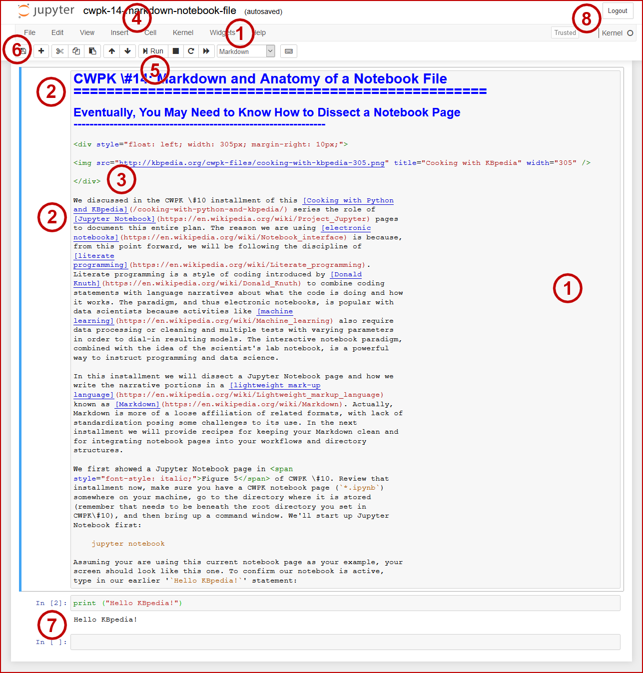
Now, scroll up to the top of this page and double-click anywhere in the area where the intro narrative is. You should get a screen like the one below, which I have annotated to point out some aspects of the interactive notebook page:

Example Markdown Cell in Edit Mode
Figure 1: Example Markdown Cell in Edit Mode

We can see that the active area on the page, what is known as a “cell” contains plain text (1). Also note that the dropdown menu in the header (1) tells us the cell is of the ‘Markdown’ type. There are multiple types of cells, but throughout this series we will be concentrating on the two main ones: Markdown for formatting narratives, and Code for entering and testing our scripts. Recall that Markdown uses plain text rather than embedded tags (as in HTML, for example) (2). We have conventions for designating headings (2) or links with URLs and link text (2). Most common page or text formatting such as bullets or italics or emphasized text or images have a plain text convention associated with them. In this instance, we are using the Pandoc flavor of Markdown. But, also notice, that we can mix many HTML elements (3) into our Markdown text to accomplish more nuanced markup. In this case, we as using the HTML <div> tag to convey style and placement information for our header with its logo.

As we open or close cells, new cells appear for entry at the bottom of our page. We can also manage these cells by inserting above or below or deleting them via two of the menu options (4). To edit, we either double-click in a Markdown cell or enter directly into a Code cell. When have finished our changes, we can see the effect via the Run button (5) or Cell option (4), including to run all cells (the complete page) or selected cells. But be careful! While we can do much entry and modifications with Markdown cells, this application is not like a standard text editor. We can get instant feedback on our modifications, but it is different to Save files as checkpoints (6) and changing file names is not possible from within the notebook, where we must use the file system. We can also have multiple cells unevaluated at a given time (7). We may also choose among multiple kernals (different languages or versions, including R and others). Many of these features we will not use in this series; the resources at the end of this article provide additional links to learn more about notebooks.

To learn more about Markdown, let me recommend two terrific resources. The first is directly relevant to Jupyter Notebook, the second is for a very useful Markdown format:

When you are done working on your notebook, you can save the notebook using Widgets → Save Notebook Widgets State OR File → Save and Checkpoint and then File → Close and Halt. (You may also Logout (8), but make sure you have saved in advance.) Depending on your sequence, you may exit to the command window. If so, and the system is still running in the background, pick Ctrl+c to quit the application and return to the command window prompt.

Should you want to convert your notebook to a Web page (*.html), you may use nbconvert at the command prompt when you are out of Jupyter Notebook. For the notebook file we have been using for this example, the command is (assuming you are in the same directory as the notebook file):

  $ jupyter nbconvert --to html cwpk-14-markdown-notebook-file.ipynb

This command will write out a large HTML page (large because it embeds all style information). This version pretty faithfully captures the exact look of the application on screen. See the nbconvert documentation for further details. Alternatively, you may export the notebook directly by picking File → Download as → HTML (.html). Then, save to your standard download location.

We will learn more about these saving options and ways to improve file size and faithful rendering in the next installment.

Important note: as of the forthcoming CWPK #16 installment, we will begin to distribute Jupyter Notebook files with the publication of each installment. Further, even though early installments in this series had no interactivity, we will also re-published them as notebook files. From this point forward all new installments will include a Notebook file. Check out CWPK #16 when it is published for more details.

More Resources

NOTE: This article is part of the Cooking with Python and KBpedia series. See the CWPK listing for other articles in the series. KBpedia has its own Web site.
NOTE: This CWPK installment is available both as an online interactive file or as a direct download to use locally. Make sure and pick the correct installment number. For the online interactive option, pick the *.ipynb file. It may take a bit of time for the interactive option to load.
I am at best an amateur with Python. There are likely more efficient methods for coding these steps than what I provide. I encourage you to experiment — which is part of the fun of Python — and to notify me should you make improvements.

Posted by AI3's author, Mike Bergman Posted on August 13, 2020 at 9:51 am in CWPK, KBpedia, Semantic Web Tools | Comments (0)
The URI link reference to this post is: https://www.mkbergman.com/2342/cwpk-14-markdown-and-anatomy-of-a-notebook-file/
The URI to trackback this post is: https://www.mkbergman.com/2342/cwpk-14-markdown-and-anatomy-of-a-notebook-file/trackback/