


 Trying to Cut Through the Terminology Confusion and Offer Simple Guidelines

Semantics is a funny thing. All professionals come to know that communication with their peers and outside audiences requires accuracy in how to express things. Yet, even with such attentiveness, communications sometimes go awry. It turns out that background, perspective and context can all act to switch circuits at the point of communication. Despite, and probably because of, our predilection as a species to classify and describe things, all from different viewpoints, we can often exhort in earnest a thought that is communicated to others as something different from what we intended. Alas!
This reality is why, I suspect, we have embraced as a species things like dictionaries, thesauri, encyclopedias, specifications, standards, sacred tracts, and such, in order to help codify what our expressions mean in a given context. So, yes, while sometimes there is sloppiness in language and elocution, many misunderstandings between parties are also a result of difference in context and perspective.
It is important when we process information in order to identify relations or extract entities, to type them or classify them, or to fill out their attributes, that we have measures to gauge how well our algorithms and tests work, all attentive to providing adequate context and perspective. These very same measures can also tell us whether our attempts to improve them are working or not. These measures, in turn, also are the keys for establishing effective gold standards and creating positive and negative training sets for machine learning. Still, despite their importance, these measures are not always easy to explain or understand. And, truth is, sometimes these measures may also be mis-explained or mis-calculated. Aiding the understanding of important measures in improving the precision, completeness, and accuracy of communications is my purpose in this article.
Some Basic Statistics as Typically Described
The most common scoring methods for gauging the “accuracy” of natural language communications involves statistical tests based on the nomenclature of negatives and positives, true or false. Sometimes it can be a bit confusing about how to interpret these terms, a confusion which can be made all the more difficult in what kind of statistical environment is at play. Let me try to first confuse, and then more simply explain these possible nuances.
Standard science is based on a branch of statistics known as statistical hypothesis testing. This is likely the statistics that you were taught in school. In hypothesis testing, we begin with a hypothesis about what might be going on with respect to a problem or issue, but for which we do not know the cause or truth. After reviewing some observations, we formulate a hypothesis that some factor A is affecting or influencing factor B. We then formulate a mirror-image null hypothesis that specifies that factor A does not affect factor B; this is what we will actually test. The null hypothesis is what we assume the world in our problem context looks like, absent our test. If the test of our formulated hypothesis does not affect that assumed distribution, then we reject our alternative (meaning our initial hypothesis fails, and we keep the null explanation).
We make assumptions from our sample about how the entire population is distributed, which enables us to choose a statistical model that captures the shape of assumed probable results for our measurement sample. These shapes or distributions may be normal (bell-shaped or Gaussian), binomial, power law, or many others. These assumptions about populations and distribution shapes then tell us what kind of statistical test(s) to perform. (Misunderstanding the true shape of the distribution of a population is one of the major sources of error in statistical analysis.) Different tests may also give us more or less statistical power to test the null hypothesis, which is that chance results will match the assumed distribution. Different tests may also give us more than one test statistic to measure variance from the null hypothesis.
We then apply our test and measure and collect our sample from the population, with random or other statistical sampling important so as not to skew results, and compare the distribution of these results to our assumed model and test statistic(s). The null hypothesis is confirmed or not by whether the shape of our sampled results matches the assumed distribution or not. The significance of the variance from the assumed shape, along with a confidence interval based on our sample size and the test at hand, provides the information necessary to either accept or reject the null hypothesis.
Rejection of the null hypothesis generally requires both significant difference from the expected shape in our sample and a high level of confidence. Absent those results, we likely need to accept the null hypothesis, thus rejecting the alternative hypothesis that some factor A is affecting or influencing factor B. Alternatively, with significant differences and a high level of confidence, we can reject the null hypothesis, thereby accepting the alternative hypothesis (our actual starting hypothesis, which prompted the null) that factor A is affecting or influencing factor B.
This is all well and good except for the fact that either the sampling method or our test may be in error. There are two types of errors that are possible: Type I errors, where a positive result corresponds to rejecting the null hypothesis; and Type II errors, where a negative result corresponds to not rejecting the null hypothesis.
We can combine all of these thoughts into what is the standard presentation for capturing these true and false, positive and negative, results [1]:
| Null hypothesis (H0) is | |||
|---|---|---|---|
| Valid/True | Invalid/False | ||
| Judgment of Null Hypothesis (H0) | Reject | False Positive Type I error |
True Positive Correct inference |
| Fail to reject (accept) | True negative Correct inference |
False negative Type II error |
|
Clear as mud, huh?
Let’s Apply Some Simplifications
Fortunately, there are a couple of ways to sharpen this standard story in the context of information retrieval (IR), natural language processing (NLP) and machine learning (ML) — the domains of direct interest to us at Structured Dynamics — to make understanding all of this much simpler. Statistical tests will always involve a trade off between the level of false positives (in which a non-match is declared to be a match) and the level of false negatives (in which an actual match is not detected) [1]. Let’s see if we can simplify our recognition and understanding of these conditions.
First, let’s start with a recent explanation from the KDNuggets Web site [2]:
“Imagine there are 100 positive cases among 10,000 cases. You want to predict which ones are positive, and you pick 200 to have a better chance of catching many of the 100 positive cases. You record the IDs of your predictions, and when you get the actual results you sum up how many times you were right or wrong. There are four ways of being right or wrong:
- TN / True Negative: case was negative and predicted negative
- TP / True Positive: case was positive and predicted positive
- FN / False Negative: case was positive but predicted negative
- FP / False Positive: case was negative but predicted positive.”
The use of ‘case’ and ‘predictions’ help, but are still a bit confusing. Let’s hear another explanation from Benjamin Roth from his recently completed thesis [3]:
“There are two error cases when extracting training data: false positive and false negative errors. A false positive match is produced if a sentence contains an entity pair for which a relation holds according to the knowledge base, but for which the sentence does not express the relation. The sentence is marked as a positive training example for the relation, however it does not contain a valid signal for it. False positives introduce errors in the training data from which the relational model is to be generalized. For most models false positive errors are the most critical error type, for qualitative and quantitative reasons, as will be explained in the following.
“A false negative error can occur if a sentence and argument pair is marked as a negative training example for a relation (the knowledge base does not contain the argument pair for that relation), but the sentence actually expresses the relation, and the knowledge base was incomplete. This type of error may negatively influence model learning by omitting potentially useful positive examples or by negatively weighting valid signals for a relation.”
In our context, we can see a couple of differences from traditional scientific hypothesis testing. First, the problems we are dealing with in IR, NLP and ML are all statistical classification problems, specifically in binary classification. For example, is a given text token an entity or not? What type amongst a discrete set is it? Does the token belong to a given classification or not? This makes it considerably easier to posit an alternative hypothesis and the shape of its distribution. What makes it binary is the decision as to whether a given result is correct or not. We now have a different set of distributions and tests from more common normal distributions.
Second, we can measure our correct ‘hits’ by applying our given tests to a “gold standard” of known results. This gold standard provides a representative sample of what our actual population looks like, one we have characterized in advance whether all results in the sample are true or not for the question at hand. Further, we can use this same gold standard over and over again to gauge improvements in our test procedures.
Combining these thoughts leads to a much simpler matrix, sometimes called a confusion matrix in this context, for laying out the true and false, positive and negative characterizations:
| Correctness | Test Assertion | |
|---|---|---|
| Positive | Negative | |
| True | TP True Positive |
TN True Negative |
| False | FP False Positive |
FN False Negative |
As we can see, ‘positive’ and ‘negative’ are simply the assertions (predictions) arising from our test algorithm of whether or not there is a match or a ‘hit’. ‘True’ and ‘false’ merely indicate whether these assertions proved to be correct or not as determined by gold standards or training sets. A false positive is a false alarm, a “crying wolf”; a false negative is a missed result. Thus, all true results are correct; all false are incorrect.
Key Information Retrieval Statistics
Armed with these four characterizations — true positive, false positive, true negative, false negative — we now have the ability to calculate some important statistical measures. Most of these IR measures also have exact analogs in standard statistics, which I also note.
The first metric captures the concept of coverage. In standard statistics, this measure is called sensitivity; in IR and NLP contexts it is called recall. Basically it measures the ‘hit’ rate for identifying true positives out of all potential positives, and is also called the true positive rate, or TPR:

Expressed as a fraction of 1.00 or a percentage, a high recall value means the test has a high “yield” for identifying positive results.
Precision is the complementary measure to recall, in that it is a measure for how efficient whether positive identifications are true or not:
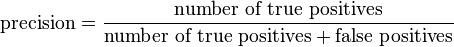
Precision is something, then, of a “quality” measure, also expressed as a fraction of 1.00 or a percentage. It provides a positive predictive value, as defined as the proportion of the true positives against all the positive results (both true positives and false positives).
So, we can see that recall gives us a measure as to the breadth of the hits captured, while precision is a statement of whether our hits are correct or not. We also see, as in the Roth quote above, why false positives need to be a focus of attention in test development, because they directly lower precision and efficiency of the test.
This recognition that precision and recall are complementary and linked is reflected in one of the preferred overall measures of IR and NLP statistics, the F-score, which is the adjusted (beta) mean of precision and recall. The general formula for positive real β is:
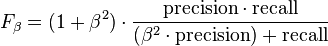 .
.
which can be expressed in terms of TP, FN and FP as:

In many cases, the harmonic mean is used, which means a beta of 1, which is called the F1 statistic:

But F1 displays a tension. Either precision or recall may be improved to achieve an improvement in F1, but with divergent benefits or effects. What is more highly valued? Yield? Quality? These choices dictate what kinds of tests and areas of improvement need to receive focus. As a result, the weight of beta can be adjusted to favor either precision or recall. Two other commonly used F measures are the F2 measure, which weights recall higher than precision, and the F0.5 measure, which puts more emphasis on precision than recall [4].
Another metric can factor into this equation, though accuracy is a less referenced measure in the IR and NLP realm. Accuracy is the statistical measure of how well a binary classification test correctly identifies or excludes a condition:

An accuracy of 100% means that the measured values are exactly the same as the given values.
All of the measures above simply require the measurement of false and true, positive and negative, as do a variety of predictive values and likelihood ratios. Relevance, prevalence and specificity are some of the other notable measures that depend solely on these metrics in combination with total population.
By bringing in some other rather simple metrics, it is also possible to expand beyond this statistical base to cover such measures as information entropy, statistical inference, pointwise mutual information, variation of information, uncertainty coefficients, information gain, AUCs and ROCs. But we’ll leave discussion of some of those options until another day.
Bringing It All Together
Courtesy of one of the major templates in Wikipedia in the statistics domain [5], for which I have taken liberties, expansions and deletions, we can envision the universe of statistical measures in IR and NLP, based solely on population and positives and negatives, true and false, as being:
| Condition (as determined by “Gold standard“) | |||||
| Total population | Condition positive | Condition negative | Prevalence = Σ Condition positive Σ Total population |
||
| Test Assertion |
Test assertion positive |
TP True positive |
FP False positive (Type I error) |
Positive predictive value (PPV), Precision = Σ True positive Σ Test outcome positive |
False discovery rate (FDR) = Σ False positive Σ Test outcome positive |
| Test assertion negative |
FN False negative (Type II error) |
TN True negative |
False omission rate (FOR) = Σ False negative Σ Test outcome negative |
Negative predictive value (NPV) = Σ True negative Σ Test outcome negative |
|
| Accuracy (ACC) = Σ True positive + Σ True negative Σ Total population |
True positive rate (TPR), Sensitivity, Recall = Σ True positive Σ Condition positive |
False positive rate (FPR),Fall-out = Σ False positive Σ Condition negative |
Positive likelihood ratio (LR+) = TPR FPR |
F-score (F1 case) = 2 x (Precision * Recall) (Precision + Recall) |
|
| False negative rate (FNR) = Σ False negative Σ Condition positive |
True negative rate (TNR), Specificity (SPC) = Σ True negative Σ Condition negative |
Negative likelihood ratio (LR−) = FNR TNR |
|||
Please note that the order and location of TP, FP, FN and TN differs from my simple layout presented in the confusion matrix above. In the confusion matrix, we are gauging whether the assertion of the test is correct or not as established by the gold standard. In this current figure, we are instead using the positive or negative status of the gold standard as the organizing dimension. Use the shorthand identifiers of TP, etc., to make the cross reference between “correct” and “condition”.
Relationships to Gold Standards and Training Sets
These basic measures and understandings have two further important roles beyond informing how to improve the accuracy and peformance of IR and NLP algorithms and tests. The first is gold standards. The second is training sets.
Gold standards that themselves contain false positives and false negatives, by definition, immediately introduce errors. These errors make it difficult to test and refine existing IR and NLP algorithms, because the baseline is skewed. And, because gold standards also often inform training sets, errors there propagate into errors in machine learning. It is also important to include true negatives in a gold standard, in the likely ratio expected by the overall population, so that this complement of the accuracy measurement is not overlooked.
Once a gold standard is created, you then run your current test regime against it when you run your same tests againt unknowns. Preferably, of course, the gold standard only includes true positives and true negatives (that is, the gold standard is the basis for judging “correctness’; see confusion matrix above). In the case of running an entity recognizer, your results against the gold standard can take one of three forms: you either have open slots (no entity asserted); slots with correct entities; or slots with incorrect entities. Thus, here is how you would create the basis for your statistical scores:
- TP = test identifies the same entity as in the gold standard
- FP = test identifies a different entity than what is in the gold standard (including no entity)
- TN = test identifies no entity; gold standard has no entity, and
- FN = test identifies no entity, but gold standard has one.
As noted before, these measures are sufficient to calculate the precision, recall, F-score and accuracy statistics. Also note that the F v T and P v N correspond to the gold standard “correctness” and what is asserted by the test(s), per the confusion matrix.
We can apply this same mindset to the second additional, important role in creating and evaluating training sets. Both positive and negative training sets are recommended for machine learning. Negative training sets are often overlooked. Again, if the learning is not based on true positives and negatives, then significant error may be introduced into the learning.
Clean, vetted gold standards and training sets are thus a critical component to improving our knowledge bases going forward [6]. The very practice of creating gold standards and training sets needs to receive as much attention as algorithm development because, without it, we are optimizing algorithms to fuzzy objectives.
The virtuous circle that occurs between more accurate standards and training sets and improved IR and ML algorithms is a central argument for knowledge-based artificial intelligence (KBAI). Continuing to iterate better knowledge bases and validation datasets is a driving factor in improving both the yield and quality from our rapidly expanding knowledge bases.
