Posted:September 15, 2014

Big Structure has a Foundation in Reference Structures, But Any Structure Aids Interoperability

Big Structure is built on a foundation of reference structures, with domain structures capturing the domain at hand. These represent the target foundations for mapping schema and transforming data in the wild into an operable, canonical form. Any structure, even the most lightweight of lists and metadata, can contribute to and be mapped into this model, as this wall of structure shows:

Foundations to Big Structure

Described below are some of these structures, in rough descending order of completeness and usefulness, for making data interoperable. Please note that any of these structures might be available as linked data.

Reference Structures

In both semantics and artificial intelligence — and certainly in the realm of data interoperability — there is always the problem of symbol grounding. In the conceptual realm, symbol grounding means that when we use a term or phrase we are referring to the same thing. In the data value realm, symbol grounding means that when we refer to an object or a number, we are referring to the same measure.

UMBEL is the standard reference ontology used by Structured Dynamics. It contains 28,000 concepts (classes and relationships) derived from the Cyc knowledge base. The reference concepts of UMBEL are mapped to Wikipedia, schema.org (used in Google’s knowledge graph), DBpedia ontology classes, GeoNames and PROTON. Similar reference structures are used to ground the actual data values and attributes.

Other reference structures may be used, so long as they are rather complete in scope and coherent in their relationships. Logical consistency is a key requirement for grounding.

Knowledge Bases

Knowledge bases combine schema with data in a logical manner; well-constructed ones support computations, inference and reasoning. To date, the two primary knowledge bases that we use are Wikipedia and Cyc. However, many specific domain knowledge bases also exist.

Knowledge bases are important sources for symbol grounding. It addition, because of their computability, they may be used with artificial intelligence methods to both extend the knowledge base and to refine the feature estimates used in the AI algorithms.

Domain Ontologies

Domain ontologies, constructed as graphs, are the principal working structures in data interoperability. Though best practices recommend they be grounded in the reference structures, the domain structures are the ones that specifically capture the concepts and data attributes of the target information domain. More effort should be focused at this level in the wall of structure than any other.

Domain structures provide unique benefits in discovery, flexible access, and information integration due to their inherent connectedness. Further, these domain structures can be layered on top of existing information assets, which means they are an enhancement and not a displacement for prior investments. And, these domain structures may be matured incrementally, which means their development is cost-effective.

Mappings

Data and schema in the wild need to be mapped and transformed into these canonical structures. What is known as data wrangling is an aspect of these mappings and transformations. Mappings thus become the glue that ties native data to interoperable forms.

Mapping is the critical bridging function in data interoperability. It requires tools and background intelligence to suggest possible correspondences; how well this is done is a key to making the semi-automatic mapping process as efficient as possible. Mapping structures are the result of the final correspondences. Mapping effort is a function of the scope of Big Structure, not the volume of Big Data.

Existing Structures

A broad variety of structures occur in the wild — from database schema and taxonomies to dictionaries and lists — that need to be represented in a common form and then mapped in order to support interoperability. The common representation used by Structured Dynamics is the RDF data model.

Structure Scripts

Scripting and tooling are essential to help create Big Structure efficiently.

Editor’s Note: We are pleased to share with you in advance some of the text from Structured Dynamics’ new Web site.
Posted:September 9, 2014

UMBEL Logo Much Clean-up, Consistency Brought to New Version

Structured Dynamics today released version 1.10 of its open source UMBEL (Upper Mapping and Binding Exchange Layer) reference concept ontology. This new release is in preparation for a series of subsequent releases planned over the next few months as additional consistency and functionality is brought to the system.

This is the first UMBEL version to be created and loaded from scratch using a new Clojure scripting framework. Fred Giasson describes these scripts and highlights some of the new functionality in a separate blog post.

Besides this new processing framework, here are the key changes at a high level made in this new version:

  • Reconciliation with the parent OpenCyc concepts
  • Added reference concept definitions where missing
  • Added additional altLabels (to the semsets) in many cases
  • Checked graph integrity for relationships between concepts
  • Reviewed and corrected prefLabels to make them unique (for more usefulness in autocompletion)
  • Checked assignments of all reference concepts to a parent SuperType
  • Reviewed SuperType assignment inconsistencies and removed some disjoint assertions
  • Updated mappings to OpenCyc, GeoNames, schema.org and the DBpedia ontology (see next).

This new UMBEL v. 1.10 is now updated and consistent with OpenCyc (version 4.0, dated October 12, 2012), GeoNames (version 3.1, dated October 29, 2012), schema.org (version 1.9, dated August 19, 2014) and the DBpedia ontology (version 3.9, retrieved August 18, 2014). The resulting mappings now are:

  • 26,091 Reference Concepts in UMBEL Core
  • 1,925 Reference Concepts in UMBEL Geo
  • 27,691 links between OpenCyc and UMBEL (which includes Core & Geo)
  • 754 links between Schema.org classes and UMBEL
  • 688 links between Geonames.org classes and UMBEL
  • 682 links between the DBpedia ontology classes and UMBEL.

These changes have also resulted in some improvements to the umbel.org Web site and its Web services, as more fully described by Fred. The updated ontologies and mappings may be found at the UMBEL GitHub site.

What’s In the Pipeline

As noted, this version update is in preparation for some pending activities, which are now moving toward completion. Subsequent releases (perhaps not in the order shown) will include:

  • Introduction of a new reference Attributes Ontology as a new module extension to UMBEL
  • Completion of the mappings to the English Wikipedia
  • Adding new concepts resulting from these Wikipedia mappings, plus adding concepts to complete 100% mappings to GeoNames, DBpedia and schema.org
  • Additional definition and semset updates to the structure
  • Checks to external mappings for consistency
  • Automated tests for completing the integrity of the UMBEL graph by identifying missing connecting concepts
  • An improved method to extend disjointedness assertions across the UMBEL structure
  • Additional Web services to support the above.

Look here and on the UMBEL mailing list for these future announcements.

Posted by AI3's author, Mike Bergman Posted on September 9, 2014 at 10:10 am in UMBEL | Comments (0)
The URI link reference to this post is: https://www.mkbergman.com/1795/umbel-version-1-10-released/
The URI to trackback this post is: https://www.mkbergman.com/1795/umbel-version-1-10-released/trackback/
Posted:September 4, 2014

Connections Attract ValueBenefits Can be Gained Incrementally, and Are Cumulative

In the earlier installments of this article series we first described how to estimate the value of connections amongst Big Data datasets, premised on the network effect. We then went into detail in the second part about the Viking algorithm (VKG) derived to capture the Value of Knowledge Graphs.

In this concluding part of the series we summarize the use and implications of the Viking algorithm on your Big Data planning. We do so by offering ten guidelines for how including Big Structure may be leveraged in the context of a knowledge graph. We then conclude the series with some caveats on the interpretation of these results and a discussion of possible future directions.

Ten Guidelines for Big Structure

As you think through your Big Data initiatives, we recommend you keep these ten guidelines relating to data structure in mind:

  1. More structure always provides benefits — adding structure always provides a multiplier effect in value
  2. Making connections is more valuable than adding more data — Big Data alone is practically worthless if not connected. Adding more records has an additive effect on the value of the datasets in comparison to the multiplier effects of structure
  3. Benefits of structure increases with increasing dataset sizes (scale) — the multiplier effect of more structure (connections) increases with scale. Big Data projects are thus perfect candidates for consciously “connecting the dots”
  4. Particular kinds of structure — such as types or categorization — have higher benefit than annotations — structural characteristics at the record level that enable cross-dataset selections and comparisons are inherently more valuable than record-specific annotations. Typing of records into entity types is a very powerful lever
  5. The potential value of a knowledge graph depends on the nature of the domain — knowing what kind of knowledge graph is in play is an important metric for being able to estimate potential value from connections. Further, by adding connections (correct and coherent) it may also be possible to move the entire structure to a lower average degree of separation (D), with further multiplier benefits
  6. Structure can be added incrementally, and is cumulative — because these additions to structure are based on the open world assumption (OWA), it is possible to add structure incrementally. OWA enables connection and structuring efforts to be accomplished as budgets allow. But, because these structural benefits are cumulative (and with multipliers), later contributions can have increasing benefits over earlier ones
  7. Data wrangling is justified as a means to increase the accuracy of fact assertions — data wrangling should not be viewed as an overall “cost” to the effort, but as a key means for achieving the multiplier benefits arising from structure and connections
  8. Adding structure at the time of data wrangling is a cost-effective approach — the corollary to standard data wrangling is the wisdom of explicitly including structuring and connection to the efforts. The multiplier benefits that accrue are a means to markedly lower the marginal costs of data wrangling in relation to realized benefits
  9. Ontologies provide inferred capabilities — though many kinds of structure can contribute to the Big Structure effort, ontologies, because of their logical structure, can be used to derive inferred “facts” in essence “for free.” (And remember, more “facts” are the basis for the multiplier benefits.) Inference provides a powerful means to leverage existing connections without explicitly needing to assert new ones
  10. Ontologies are the most preferred means for Big Structure — besides inference, ontologies set a structural framework of relationships (schema) very useful to helping to guide the nature of connections made. Also, ontologies can provide the conceptual and descriptive richness useful for tagging and other structure-adding activities [1]. Because of these advantages and their testable nature based in logic, ontologies represent the pinnacle of structural forms to achieve these value benefits.

Of course, mere connections for structure’s sake is silly. It is important that the structure added and connections made are correct, consistent and coherent. Even then, not all types of connections are created equal, with typing the most important, annotations the least.

The good thing is that Big Structure can be added as a slight increase over standard data wrangling efforts, and with much greater impact than standard wrangling. Further, the structures themselves, preferably guided by domain ontologies, are a means of testing these factors for subsequent structure additions. Not only does adding structure get easier with a foundation of existing structure, but it increases the value of the information by orders of magnitude.

Not the Last Word

Roughly twenty years ago Metcalfe’s law triggered a gold rush in trying to achieve network effects at Internet scale. Though the algorithm proved too optimistic at larger scales, the idea of the benefit from connections was firmly established. Ten years ago it was clear that some form of diminishing returns needed to be applied to connections at scale. Zipf’s law was not a bad guess, though we have subsequently learned that more graph-centric measures are more appropriate and accurate for estimating value. Now, the Viking algorithm has emerged as the best estimator of the value of connections within Big Data.

I suspect we will see further improvements to the Viking algorithm as: 1) we come to better understand graph structures (including the effects of clusters and cliques); and 2) we learn to distinguish the different value of different types of connections [2]. We can already see that typing and categorization have better structural effects above annotations. We further can see that the correctness of asserted “facts” is a key to realizing the multiplier benefits of connections and structures. Thus, we should see improved means for screening and testing assertions for their accuracy at scale.

At this stage, what the Viking algorithm gives us is a defensible means for assessing the value of adding structure (through connections) to our datasets. We see these multiplier effects to be huge, and to compound to even still further benefits with scale. We also see that the most developed forms of structure — namely, ontologies — bring still further benefits in inference and testable coherence. All Big Structure efforts should be aiming to express all of the structural insights for the organization and its datasets into these ontological forms [1].

While our current proxy for value — namely, asserted “facts” — is useful, it would also be helpful to be able to translate these “fact” assertions into a monetary value. As we move down this path we will discover, again, that not all “facts” are created equal, and some have more monetary value than others. Transitioning our estimates of value to a monetary basis will help set parameters for the cost-benefit analysis of data collection and structurizing that is the ultimate basis for planning Big Data and Big Structure initiatives.

In the end, many things need to be analyzed to understand the impacts of each connection and structure metric on the value of the resulting graph. But, what today’s current understanding of the network effect and the Viking algorithm brings us is a better means to understand and quantify the benefits of connected information. By any measure, these value benefits are multiples of what we see for unconnected data, the multiples of which grow massively with the scale of the data and their connections.

Big Structure is fertile ground for bringing in the sheaves. Let the harvesting begin.


[1] Though not further discussed here, the ontologies also provide the means for tagging (providing structure) to unstructured documents, which also brings the multiplier benefits from structure. On the retrieval side, such structure also aids faceting and filtered “slicing and dicing” of underlying datasets, thereby improving retrieval efficacy.
[2] As one of the first approaches to capture these nuances, see Mischa Dohler, Thomas Watteyne, Fabrice Valois and Jia-Liang Lu, 2008. Kumar’s, Zipf’s and Other Laws: How to Structure a Large-Scale Wireless Network?, published in Annales des Telecommunications – Annals of Telecommunications 63, 5-6 pp. 239-251. See http://hal.archives-ouvertes.fr/docs/00/40/58/67/PDF/Large_Scale_Networks_journal_FINAL.pdf.
Posted:September 3, 2014

Value of Connecting ThingsPart II of The Value of Connecting Things: Big Structure Improves Big Data by Orders of Magnitude

Yesterday in the first part of this series we raised the important question of how to value connections made between data. At the Big Data scales represented, we prepared a Basic Facts case of up to 2 billion assertions. We are using asserted “facts” as our value proxy. We’ll talk more about value and caveats in the third part of our series, tomorrow.

We saw that early estimates of network effects, such as Metcalfe’s law, overestimate value at scale. We looked at Zipf’s law as a means to capture the diminishing value of connections given the distance between facts. In today’s article we will focus on these factors of interaction and potential value in the specific context of knowledge graphs. Knowledge graphs are Big Structure representations that capture the schematics, concepts and measures in any given knowledge domain (that is, any domain of human activity).

Since I first tried to address the value of knowledge networks some five years ago [1], I have been disturbed about a couple of things [2]. First, I felt that the exponential or geometric bases for estimating the value of information connections were not correct, both because they fail at scale and they don’t discriminate that some connections work and are more important, while others are trivial or don’t work. Capturing this law of diminishing value in a context that makes sense for knowledge bases was, I felt, the key to answering the value riddle.

I believe we have now, in this series, provided a compelling basis for solving that riddle, which also points the way to further improvements. This assertion is an exciting statement, in that we now may have a quantitative basis in hand for determining where and how to spend our monies for Big Data and Big Structure initiatives. Such quantitative tools are a huge boon to bring analytic rigor to the data collection and integration challenge.

Adding connections (“Big Structure“) to Big Data can increase the value of enterprise information from one to three orders of magnitude; the value also scales linearly with added structure (attributes).

This article shows that adding connections (“Big Structure“) at Big Data scales can increase the value of enterprise information from one (ten) to three (thousands) orders of magnitude. The magnitude of the value scales linearly with each added structure (attribute). These value multipliers from adding Big Structure are a tremendously cost-effective addition to standard data wrangling efforts.

The Value of Knowledge Graphs (VKG) Formulation

The recognition of the need for a law of diminishing returns to reflect the distance between facts or assertions is a central argument in the Briscoe-Odlyzko-Tilly formulation (see [3] directly, and the prior Part I discussion). Not all information is connected, and not all connected information is of equivalent worth. The implied question in these statements, however, is how to capture those differences?

The B-O-T (or sometimes, O-T) formulation does not choose a bad starting proxy for this diminishment law. Zipf’s law reflects many observed distributions in human objects, roughly equivalant to power law, Pareto (“80:20”) distributions or n log (n) diminishing returns with long-tail characteristics. Examples include Internet distributions (such as popularity of Web sites or search terms), human language distributions, income rankings, population distributions, etc. There is no question that Zipf’s law distributions are common and frequent.

The only problem with picking the Zipf’s law basis, however, is that there was absolutely no evidence that such occurred for information networks or knowledge graphs. Zipf’s law distributions tend to be statements across single types for a single attribute distribution. Graphs, we can safely say, are anything but this distribution. Connections and multiple types are the rule, not the exception.

So, maybe the B-O-T formulation was correct, and maybe it was not. There was no empirical evidence to support this assertion for knowledge graphs. And, there did not appear to be a compelling logic argument for relating Zipf’s law to graphs other than they are artifacts of human endeavor.

My discomfort in adopting this arbitrary B-O-T basis, even though solidly embedded in human experience, caused me to seek alternative ideas and explanations, but also ones that fulfilled the key structural insights of diminishing returns and non-equivalent assertions that were the focal points of B-O-T, all within a graph context.

The Starting Basis

The breakthough occurred when I discovered an obscure, un-cited paper by Yaakov Stein [4]. Stein, a network and signals processing researcher of the first rank [4], wrote his paper as a means to understand and quantify his experience of joining LinkedIn and expanding his network. He began without an account and documented his experience as he joined and expanded his network of contacts on LinkedIn. He charted direct links, and then meticulously looked at and recorded secondary and tertiary links.

His formulation recognized that the value to an individual user equaled raising the access to the entire network (1) for that user plus the diminishing benefit represented by the participating graph’s other participants as measured by average degree of separation (d). d is an inherent measure of the graph type.

Though his context was a social network, the basic observation obtains: relations diminish by distance within a graph, with average link distance (directly related to degree of separation) being the key relevance metric. Connected “facts” or “friends” is essentially the same thing. It is all about what is shared amongst graph nodes.

The usefulness of this approach is that it grounds the multiplier effect in an inherent characteristic of the source graph, its average degree of separation [5]. Like Zipf’s law, the degree of separation is a distance measure, but one grounded specifically in graphs. Here is the Stein formulation:

Stein Formulation

A graph with a degree of separation of 4, then, would exhibit a network-wide power factor of 5/4 (4/4 plus 1/4).

The Viking Algorithm

As applied to knowledge graphs, however, this formulation still has two problems. The first minor one is that the degree of separation parameter should be D (the average across structure) rather than d. The second substantive one is that a correction factor needs to be included that accounts for the probability that an assertion may be false. This factor, F, is 1 – the measured error rate.

The resulting algorithm we term the Value of Knowledge Graph formulation, or the VKG (Viking) algorithm. It is expressed like this:

Value of Knowledge Graphs

F is meant to be analogous to F-measure, the combined precision and recall statistic for information retrieval and NLP tasks. F in the case of the Viking algorithm is also meant to be a combined statistic that represents the “accuracy” (verifiable truthfulness) of statements asserted in the graph. F is essentially an estimated value for the residual falsity for the average statement in a graph, after removal of all assertions that do not meet existing coherency, consistency or completeness tests. F is determined by sampling statements across the graph and manually testing for truthfulness (or in a logical sense, validity given the existing statements in the graph). An F of 1 signifies complete truthfulness (accuracy); an F of 0 represents complete falsity [6].

Viking in Relation to Other Network Estimators

Now, with this explanation of basis, we can again look at the value of the Viking (VKG) algorithm in comparison to those discussed in the first part of this series. Again on a logarithmic scale, here are those results:

Knowledge Network Estimates

Figure 1. Knowledge Network Estimates

Excluding the exponential and geometric multipliers (namely, the “laws” of Metcalfe and Reed) in the top two curves, this shows the Viking (VKG) algorithm to have higher value than the B-O-T (O-T) algorithm, both of which are considerably higher than the Basic Facts. However, because the Figure 1 above has a logarithmic scale, these differences are harder to discern.

Viking Benefits Over the Basic Facts

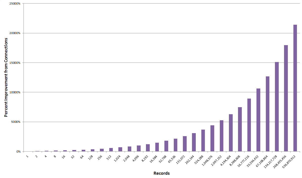
Now corrected with our assumed F factor, we can begin to tease out the value benefits of connecting “facts” versus the unconnected Basic Facts. As with any logarithmic function, we see that the value benefits from connections increase in a growing manner at larger scales. For example, as Figure 2 shows below, at a level of 1000 records, the benefits from connections are 7x greater than unconnected data. By the time the scale grows to 1 million or 500 million records, the value benefits of connections grows to 44x to 215x, respectively:

Percent Improvement from Connections

Figure 2. Percent Improvement from Connections Scales with Records Size

Benefits from connections increase as a power function at increasing scales.

Setting the VKG Factor D

But the potential value of connectedness is also a function of the general degree of information separation for the given domain. We are still in the early phases of gathering statistics for such things, but the table below summarizes what is known about the “standard” level of connectivity in various domains and applications. Note, in general, most any knowledge graph would have a D factor ranging from 2 to 8:

Category Degrees of Separation (D) Notes
Food webs ~ 2 [7]
Genetic differences ~ 3 [8]
LinkedIn ~ 3 [4]
Twitter 3.435 – 4.67 [9]
Facebook 3.74 [10]
Potential research collaborators ~ 4 [11]
UMBEL ~ 5.2 [12]
Social networks (general) ~ 6
Mobile ad hoc networks ~ 7 [13]
Small-world networks (max) ~ 8 [14]
Table 1. Degrees of Separation for Various Knowledge Networks

More tightly linked, cohesive domains tend to have the lower degrees of separation. It is also interesting to note that some social networks, like Twitter and Facebook, are also able to lower degrees of separation (in comparison to their nominal “social network” benchmark) by virtue of the nature of their service.

As experience is gained and with more research, I expect more estimates and more refined ones. Depending on the nature of the domain at hand, it should then be possible to pick the closest analog to use in the Viking valuation algorithm. Nonetheless, we already have a range and respective values to provide meaningful value estimates today.

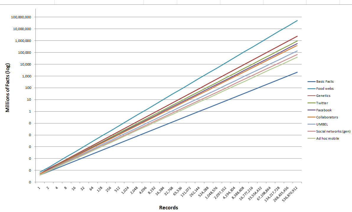
Using the values in Table 1, we are thus able to plot the effects (again, log scale) of these various degrees of separation in terms of the “fact” assertions that can be made for our Big Data test dataset:

Potential Network Value Varies by Domain

Figure 3. Nature of Knowledge Graph Affects Potential Network Value

At the nominal Big Data scales of 100,000 and 1,000,000 records, the value of data connections in comparison to the unconnected Basic Facts case shows these following value improvement multipliers:

Domain 100,000 Records 1,000,000 Records
Food webs 203x 611x
Genetic differences 38x 84x
Twitter 23x 46x
Facebook 17x 33x
Potential research collaborators 14x 26x
UMBEL 8x 12x
Social networks (general) 5x 8x
Mobile ad hoc networks 3x 5x
Table 2. Multiplier (X) Improvements by Domain from Connections Over the Basic Facts

Of course, our “Big Data Example” from Part I was silent about the exact nature of its knowledge graph. Based on empircial experience to date, the benefits from connecting data that was previously unconnected should fall somewhere within the limits of Table 2. Even at rather low scales and more loosely-connected domains, the value improvements in making connections with data is many-fold. At larger scales for tighter networks, the multipliers can become astounding.

Adding Structure to the Underlying Data

Another implication that the Viking algorithm allows us to test is the comparative benefit from adding structure to our datasets. Actually, “adding structure” is not strictly correct; it is “structurizing” the data via characterizations, attributes and categorizations. Of course, not all structure is created equal. Assigning or classifying our records into types, for example, applies to all records across the datasets and provides powerful cross-record linkages. Adding annotations or metadata to single records provides much lower benefits.

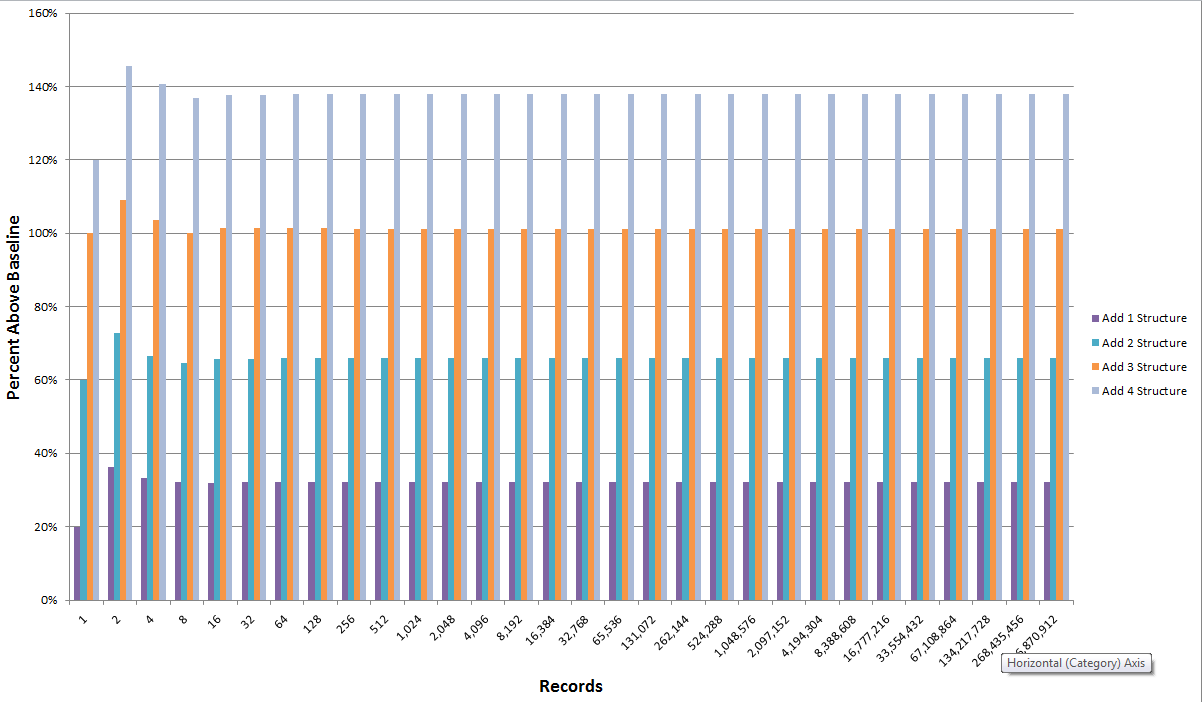
When we add structure across datasets the value improvements are a linear percent, as this figure shows:

Adding Structure has a Linear Effect on Value

Figure 4. Adding Structure has a Linear Effect on Value

For our Big Data example, each across-dataset structure characterization adds about 25% to 30% value per structure. Adding four structural characterizations, for example, more than doubles the “facts” assertion value (~ 140%) to the datasets.

Preview of Last Part

The last part forthcoming tomorrow will summarize the implications from the Viking algorithm on the role and importance of Big Structure to your organization’s Big Data efforts. Some caveats and future directions will conclude the series.


[1] The two articles written at that time were, M.K. Bergman, 2009. Structure the World, in AI3:::Adaptive Information blog, August 3, 2009, and M.K. Bergman, 2009, The Law of Linked Data, AI3:::Adaptive Information blog, October 11, 2009.
[2] See also the then-current state of analysis by Eric Hellman, 2009. Normal and Inverse Network Effects for Linked Data, published in his blog, October 15, 2009; see http://go-to-hellman.blogspot.com/2009/10/normal-and-inverse-network-effects-for.html.
[3] Bob Briscoe, Andrew Odlyzko, and Benjamin Tilly, 2006. “Metcalfe’s Law is Wrong,” in IEEE Spectrum, July 2006. A copy may be viewed at http://www.cse.unr.edu/~yuksem/teaching/nae/reading/2006-briscoe-metcalfes.pdf. Odlyzko, and Tilly had published an earlier version, (sometimes the approach is shown as O-T in addition to B-O-T), and the basic form of the algorithm appears in a single Odlyzko paper.
[4] Yaakov (J) Stein, 2009. The Value of Being Linked In, on his personal Web site, April 2009; see http://www.dspcsp.com/pubs/linkedin.pdf. Note that his empirical tests suggested a degree of separation for LinkedIn of 3.
[5] The average degree of separation is simply the graph’s average path distance – 1. For an explanation of average path distance, see [12].
[6] F is a summed average value across all assertions within a knowledge graph. In information retrieval, F-measures are now being achieved that exceed 0.90 (90%). For the cases used herein, F is estimated at 0.85. Again, this parameter is measured after all standard coherency, consistency, and completeness tests are applied to the ontology. These tests routinely remove many false assertions and establish the basic integrity of the graph. This acceptance threshold is itself constantly improving as experience is gained with basic graph integrity tests. In other words, tomorrow’s thresholds will be higher than today’s.
[7] Richard J. Williams, Eric L. Berlow, Jennifer A. Dunne, Albert-László Barabási, and Neo D. Martinez, 2002. Two Degrees of Separation in Complex Food Webs, in Proceedings of the National Academy of Sciences, 99 (20):12913-12916, September 16, 2002, doi:10.1073/pnas.192448799; see http://www.pnas.org/content/99/20/12913.full.
[9] Reza Bakhshandeh, Mehdi Samadi, Zohreh Azimifar and Jonathan Schaeffer, 2011. Degrees of Separation in Social Networks, in Proceedings, The Fourth International Symposium on Combinatorial Search (SoCS-2011), 6 pp.; see http://www.aaai.org/ocs/index.php/SOCS/SOCS11/paper/viewFile/4031/4352; and Haewoon Kwak, Changhyun Lee, Hosung Park, and Sue Moon, 2010. What is Twitter, a Social Network or a News Media?, in Proceedings of the 19th International Conference on World Wide Web, April 26–30, 2010, Raleigh, North Carolina, pp. 591-600, ACM; see http://snap.stanford.edu/class/cs224w-readings/kwak10twitter.pdf.
[10] Lars Backstrom et al., 2012. Four Degrees of Separation, Archiv.org, January 6, 2012; see http://arxiv.org/pdf/1111.4570.pdf.
[11] Paweena Chaiwanarom, Ryutaro Ichise, and Chidchano Lursinsap, 2010. Finding Potential Research Collaborators in Four Degrees of Separation, pp. 399-410, in Longbing Cao, Jiang Zhong, and Yong Feng, eds., Advanced Data Mining and Applications, Springer Berlin Heidelberg, http://dx.doi.org/10.1007/978-3-642-17313-4_39.
[13] Maria Papadopouli and Henning Schulzrinne, 2000. Seven Degrees of Separation in Mobile ad hoc Networks, presented at Global Telecommunications Conference, 2000 (GLOBECOM’00), IEEE. Vol. 3; see http://www.huaxiaspace.net/academic/classes/wi02/cse294/20020222globecom2000.pdf.
[14] Paolo Pin, 2006. Eight Degrees of Separation, in Nota di Lavoro, Fondazione Eni Enrico Mattei, No. 78.2006 see http://www.econstor.eu/bitstream/10419/74249/1/NDL2006-078.pdf.
Posted:September 2, 2014

Value of Connecting ThingsTeasing Out the Role of Big Structure in Context and Connections

The hackneyed phrase of “connect the dots” reflects our basic intuition that there is value in making connections amongst relevant data. But, what is this value? How might we quantify it? This topic, and a method and guidelines for doing so, are the subject of this article and the second and third parts to follow.

The reason it is important to quantify the value of connected information is that such an estimate helps to define what effort or cost we can justify in order to derive those connections. In Big Data, for example, we already know that 50% to 80% of the costs in assembling relevant datasets is due to data wrangling — the effort to extract, transform and clean the input data [1]. No where, however, do we know what it is worth to go to the next step of working to connect those data.

Quantifying this understanding will thus also help determine what the value is in developing Big Structure, the approach we have been most recently discussing for how to organize and connect Big Data. Big Structure sets the schematic and data relationships for how data from disparate sources can be connected together.

About five years ago I wrote my first articles on how we might approach the quantification of these information connections [2]. That first, cursory look was useful for bounding the problem, but no firm conclusions as to how to specifically quantify this value were proposed. Like other graphs or networks, the usefulness of the ‘network effect‘ to bound the question was clear. It has taken further research and experiences with actual linked datasets to point to how to resolve this quantification challenge.

Foundations in the Network Effect

The network effect was first realized in the early days of telephone networks, where the value of the system increased as a function of more users [3]. We have also long recognized a similar effect in connecting information together and the breaking down of information or ‘data silos‘. As the following diagram shows, unconnected data nodes or silos look like random particles caught in the chaos of Brownian motion:

Linked Data Law Network Effect

Figure 1. ‘Network Effect’ for Connected Data

As initial connections get made, bits of structure begin to emerge. But, as connections are proliferated — analogous to the network effects of connected networks — coherence and more structure emerge.

This emergence of structure is particularly evident in physical networks, such as the growth of this hypothetical telecommunications network:

Metcalfe Law Network Effect

Figure 2. ‘Network Effect’ for Telecommunications Networks

This diagram, modified from Wikipedia to be a horizontal image, shows how two telephones can make only one connection, five can make 10 connections, and twelve can make 66 connections, etc. It is this very multiplier effect that has led to most of the thinking of how to quantify the network effect.

We can see an interesting parallel between telecommunications networks and knowledge graphs. In the telecommunication network, the addition of a new user (node) by definition brings with it connections. This is what is shown in Figure 2. But in information silos, the information is already there (nodes, or the left-side of Figure 1); what is missing are the connections (the right-side of Figure 1). By explicitly adding connections we can also create network effects, as others have noted [4].

However, once we understand these parallels, we must also recognize the differences. To properly estimate the network effects of knowledge graphs, we must be explicit about the similarities and differences with other (physical) networks [5].

Objectives for a Knowledge Graph Formulation

Since our objective is to quantify the “value” of a knowledge graph, we must first ask what is the basis of this value. In the best of all worlds, we would know the monetary worth of information, so we could justify what to spend in order to leverage it, which of course varies wildly across bases and sources. But we don’t. We do know, however, that a knowledge graph and the information it connects to constitutes a knowledge base. In the context of a knowledge base, the measure of value is the number of “correct” facts it contains. Therefore, we will use the number of connections in the graph (equivalent to the number of triple statements) as a proxy for value, representing the asserted “facts” of the graph.

We will also seek measures of graph distance and connectedness to capture the network-like qualities of the knowledge base. The characteristics of the graph itself should be the input base upon which to estimate value.

Alternative Estimates of the Network Effect

The earliest effort to estimate the value of physical networks was Sarnoff’s law, developed by David Sarnoff, for many years the leader of the Radio Corporation of America (RCA). He posited that the value of a broadcast network was directly proportional to its number of viewers (n). However, the problem with this formulation is that a broadcast network is only one way, from broadcaster to user. What of networks where there is interaction or two-way linkages? The benefits of such networks must surely be more than linear.

Once we get into interaction effects we get into multipliers. And the proper nature of those multipliers must come from the nature and extent of those interactions, as well as perhaps the nature of the network itself. I discuss below some of the more prominent candidates that have been put forward for estimating the network effect, or the value of networks.

Metcalfe’s Law

Metcalfe’s law was the first direct derivation from the telecommunications model. Robert Metcalfe formulated it about 1980 in relation to Ethernet and fax machines; the “law” was then named for Metcalfe and popularized by George Gilder in 1993. The actual algorithm proposed by Metcalfe calculates the number of unique connections in a network with n nodes to be n(n − 1)/2, which is proportional to n2. This makes Metcalfe’s law a quadratic growth equation.

The law is generally simplified [6] to state that the value of a telecommunications network is proportional to the square of the number of users of the system (n²):

Metcalfe's Law

Gilder’s popularization and the early growth of the Internet made the estimation of the benefits of network effects a very timely topic. For example, as a value measure, the network effect could be used to estimate the benefits for larger and larger numbers of users. Some have even blamed Metcalfe’s law for contributing to the creation (and then bursting) of the “dot-com bubble” of the late 1990s [7].

Metcalfe’s law clearly showed that interaction effects between nodes could generate multipliers that scaled rapidly with increasing numbers of nodes (users).

Reed’s Law

From a different perspective and with a different take, David Reed came up with a multiplier formulation that is the largest presented — anywhere. Reed’s context is social groups, and from that perspective he can envision arbitrary sized groups forming amongst any and all participants (nodes). Because of this theoretical, global scope, justified through examples such as eBay and chat rooms, Reed specifically defined group-forming networks (GFNs), as the applicable scope [8]. The simplified formulation for Reed is:

Reed's Law

In scope and context, Reed does not apply to knowledge graphs, and even in the areas of social groups, most researchers find the exponential implications of Reed’s law unsupportable [9]. The next group, for example, offers direct criticism.

Briscoe – Odlyzko – Tilly Formulation

Under the provocative title, “Metcalfe’s Law is Wrong,” Briscoe, Odlyzko, and Tilly challenged both the Metcalfe and Reed approaches in 2006 [10]. Using the proxy of Internet valuation, the authors were able to show how impractical the implications of either approach were at scale. Like the bet of rice (or wheat) doubling each of the 64 squares on a chessboard bankrupting the kingdom, the exponential implications of these two “laws” can be seen to (eventually) violate common sense.

The fundamental fallacy associated with both the Metcalfe and Reed approaches is that all potential links are of equal value [10]. But no where in the real world do we see this to be true. There must be some law of diminishing returns that must be applied to slow the unsustainable rates of exponential or (to a lesser extent) quadratic growth.

After much hand waving, the authors chose Zipf’s law as their basis for this diminishing return. The increasing “decay rate” with distance is a common distribution pattern for real-world datasets, which Zipf’s law specifically addresses, always showing power law distributions with long tails. To approximate this distribution they offered the simple n log (n) formulation of Zipf’s law [11].

Briscoe-Odlyzko-Tilly Formulation

This is a reasonable approximation, but one that is never related directly to the nature of graphs or networks. That is the source of the next layer of refinements.

VKG Formulation

I will discuss this algorithm, our recommended formulation, in Part II of this series.

A Big Data Example

In order to discuss further the question of value arising from network effects, we need a case study example. We also need to define “value”, which in this case study example, as also noted above, means the number of “facts” or assertions in our database [12]. This we call the Basic Facts (“assertions”) column.

For our basic “facts”, we consider a data series that is doubling in size for each step, eventually reaching a half billion records. Each record has four attributes or characterizations, leading to a total of more than 2 billion “facts” in the database. These are the first two columns in this table:

Records Basic Facts (“assertions”) Big Data Example
1 4 4
2 8 8
4 16 16
8 32 32
16 64 64
32 128 128
64 256 256
128 512 512
256 1,024 1,024
512 2,048 2,048
1,024 4,096 4,100
2,048 8,192 8,200
4,096 16,384 16,400
8,192 32,768 32,800
16,384 65,536 65,600
32,768 131,072 131,200
65,536 262,144 262,404
131,072 524,288 524,812
262,144 1,048,576 1,049,624
524,288 2,097,152 2,099,248
1,048,576 4,194,304 4,198,496
2,097,152 8,388,608 8,396,996
4,194,304 16,777,216 16,793,992
8,388,608 33,554,432 33,587,984
16,777,216 67,108,864 67,175,972
33,554,432 134,217,728 134,351,944
67,108,864 268,435,456 268,703,888
134,217,728 536,870,912 537,407,780
268,435,456 1,073,741,824 1,074,815,564
536,870,912 2,147,483,648 2,149,631,128
Table 1. Basic Facts Connections with a Big Data Example

At this point, we have no connections between records. Each record has four attributes each, in isolation. This basis is akin to the unconnected dots on the left side of Figure 1 above.

For our Big Data Example, we will posit a record matching procedure as our first task for a new Big Data initiative. The assumption is that across all records, one-in-10000 matches another record. This results in the number of assertions (“facts”) shown in the third column in the table above. The posited Big Data initiative results in a 0.10% increase in “facts”, irrespective of record scale, once the matching threshold is reached. This result is not terribly impressive, but is perhaps not too unrelated from a first foray into a Big Data project.

Note that the following charts and analyses (including in the next part tomorrow) use as their “Basic Facts” the number of “assertions”, or the middle column in the table above. Though Big Data may represent an initial 0.10% improvement over this, that is immaterial to what our Big Structure viewpoints will provide. So, our “Basic Facts” will be unconnected records.

Applying Network Effects to the Basic Facts

We can now apply our various network effect estimators to this base case. And, because of the fast-compounding nature of both the Reed and Metcalfe approaches, we need to plot this out on logarithmic scale [13] (click to enlarge):
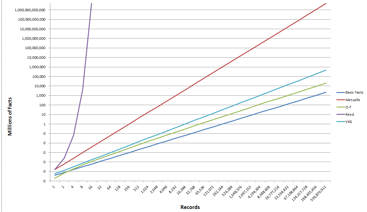
Knowledge Network Estimates

Figure 3. Knowledge Network Estimates

On a logarithmic scale, the O-T (Briscoe-Odlyzko-Tilly) and VKG formulations appear only marginally better than the Basic Facts base case, but that is only due to the swamping effects of the unrealistic growth multipliers. We’ll get into this more tomorrow.

Preview of Next Part

The next part forthcoming tomorrow will use this foundation to describe the VKG algorithm, and some of implications of its characteristics, all in the context of knowledge networks or graphs.


[1] “Data scientists, according to interviews and expert estimates, spend from 50 percent to 80 percent of their time mired in this more mundane labor of collecting and preparing unruly digital data, before it can be explored for useful nuggets,” is a quote from Steve Lohr, 2014, “For Big-Data Scientists, ‘Janitor Work’ Is Key Hurdle to Insights,” August 17, 2014, New York Times, see http://www.nytimes.com/2014/08/18/technology/for-big-data-scientists-hurdle-to-insights-is-janitor-work.html. Also, as another example of the common 80% estimate for data preparation costs, see http://radar.oreilly.com/2013/09/data-analysis-just-one-component-of-the-data-science-workflow.html.
[2] These two articles were, M.K. Bergman, 2009. Structure the World, in AI3:::Adaptive Information blog, August 3, 2009, and M.K. Bergman, 2009, The Law of Linked Data, AI3:::Adaptive Information blog, October 11, 2009. The same concerns I had at that time in the current state of analysis was captured by Eric Hellman, 2009. Normal and Inverse Network Effects for Linked Data, published in his blog, October 15, 2009; see http://go-to-hellman.blogspot.com/2009/10/normal-and-inverse-network-effects-for.html.
[3] These network effect benefits were reportedly a major driver of Theodore Newton Vail‘s efforts to consolidate the thousands of initial telephone networks in the United States under the banner of the American Telephone & Telegraph (Ma Bell) company.
[4] See, for example, James Hendler and Jennifer Golbeck, 2008. Metcalfe’s Law, Web 2.0, and the Semantic Web, in Web Semantics: Science, Services and Agents on the World Wide Web 6(1): 14-20; see http://www.cs.umd.edu/~golbeck/downloads/Web20-SW-JWS-webVersion.pdf.
[5] Babak Hodjat and Adam Cheyer, 2003. Evolution of the Laws that Deal with the Utilization of Information Networks, in Masoud Nikravesh, Lotfi A. Zadeh and Janusz Kacprzyk, eds., Studies in Fuzziness and Soft Computing, Vol 164/2005, pp. 427-438, Springer, Berlin. See http://www.adam.cheyer.com/papers/KnowledgeNetworks_Formatted.pdf.
[6] For a well-connected network, every node (n) connects to every other node (n-1), which gives us n*(n-1) or (n2n). Working this out, two nodes have two connections (2*2 – 2), three nodes have six connections (3*3 – 3) and the expression converges on the square of ‘n’ for larger values of ‘n’, e.g., (100*100 – 100) is 99% of (100*100). This convergence at larger number is the basis for the exponential simplification, 2n. Most of the other ‘laws’ stated herein are simplifications in a similar manner.
[7] See, for example, Sara F. Peralta, 2011. Moore’s Law, Metcalfe’s Law, and the Dot Com Bubble, November 27, 2011, see https://storify.com/sarafperalta/moore-s-law-metcalfe-s-law-bubble. Also see [10].
[8] David P. Reed, 1999. That Sneaky Exponential—Beyond Metcalfe’s Law to the Power of Community Building, August 27, 1999; online at http://www.reed.com/dpr/locus/gfn/reedslaw.html. For original version, see http://contextmag.com/archives/199903/digitalstrategyreedslaw.asp. Like Metcalfe, at smaller numbers the actual formula is 2nn – 1, which rapidly converges to 2n.
[9] However, one group has published an alternative formulation consistent with the Reed approach; see Kalevi Kilkki, and Matti Kalervo, 2004. KK-law for Group Forming Services, in XVth International Symposium on Services and Local Access, Edinburgh, March 2004. See http://kotisivukone.fi/files/50ajatelmaa.ajatukset.fi/tiedostot/Others/kilkki_kk-law.pdf.
[10] Bob Briscoe, Andrew Odlyzko, and Benjamin Tilly, 2006. “Metcalfe’s Law is Wrong,” in IEEE Spectrum, July 2006. A copy may be viewed at http://www.cse.unr.edu/~yuksem/teaching/nae/reading/2006-briscoe-metcalfes.pdf. Odlyzko, and Tilly had published an earlier version, (sometimes the approach is shown as O-T in addition to B-O-T), and the basic form of the algorithm appears in a single Odlyzko paper.
[12] In specific terms, each “fact” in our knowledge base is an assertion, represented as an RDF triple statement. Because some of these assertions may not, in fact, be true, the use of “fact” does not imply universal truthfulness. Rather, an assertion that passes current tests for logic, coherency, consistency or completeness is what is retained, even though its truthfulness is not certain. Therefore, separate adjustment factors (parameters) need to be applied to address accuracy tests.
[13] We adjusted the scale further to reduce the exponential absurdity of the Reed approach by manually shifting the scale downward. As a result, the Reed approach exits the chart rather quickly, heading straight up.

Posted by AI3's author, Mike Bergman Posted on September 2, 2014 at 9:10 am in Big Structure, Enterprise-scale Semantic Systems, Ontologies | Comments (0)
The URI link reference to this post is: https://www.mkbergman.com/1788/the-value-of-connecting-things-part-i-a-foundation-based-on-the-network-effect/
The URI to trackback this post is: https://www.mkbergman.com/1788/the-value-of-connecting-things-part-i-a-foundation-based-on-the-network-effect/trackback/