Let’s Get More Familiar with Python Syntax and Jupyter

Now that we have our basic environment set up and working, it is time to become a bit familiar with Python code and programs. To do so, we will use some online and reference documentation, relying in particular on an interaction environment with our Jupyter Notebook. In fact, from this point forward, all of our installments in the Cooking with Python and KBpedia series will also be accompanied by a working *.ipynb Notebook file that you are free to download and interact with at your leisure. Availability of the interactive notebooks will begin on Monday with CWPK #16.

Here are three interactive guides on how to program in Python using the interactive Jupyter Notebook environment. You may find use from all three (and there are many more on the Web, see especially GitHub and search on ‘jupyter python tutorial’, no quotes). I list these in suggested order for download and investigation if your time is limited:

1. An Introduction To Scripting in Python 3 – a good starting point with short, crisp lessons [1]
2. Python 3 Tutorial Using Jupyter Notebook – an update to Python3 from a well-regarded earlier Python2 guide [2]
3. An Introduction to Python and Programming – a 28-part notebook series. [3]

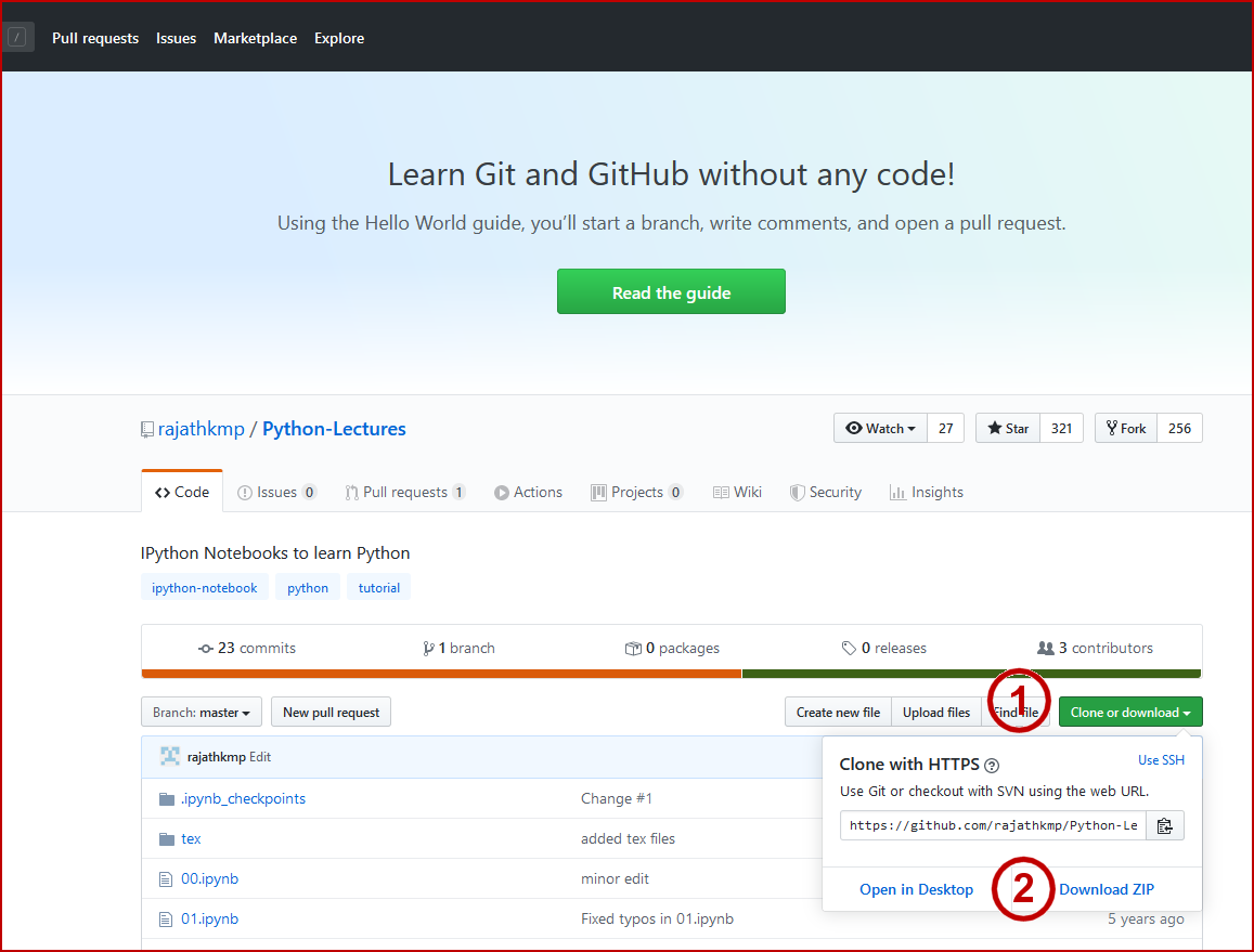
To download these from GitHub, go to the respective linked sites and pick the Clone or download button (1), followed by Download ZIP (2):

And save the *.zip files to a location of your choosing (see further below). (Recall we are punting on the question of GitHub ‘pull’ requests in this series.) Unzip the downloads to their respective directories. We are now ready to start the Jupyter Notebook.

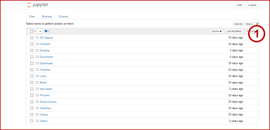
Recall that we may launch the Jupyter Notebook from either the Anaconda Prompt (CWPK #11) or from the Anaconda Navigator (CWPK #10). If we are launching from the prompt, the command is (base) C:\Users\user\jupyter notebook. Upon launch we see the standard Jupyter Notebook entry screen using the default C:\Users\user\ location used by the program:

If you play around with that directory structure, you will notice that this default directory is the root, and you are unable to navigate above it in your local file system. That poses a problem for me personally. I have for years not accepted Microsoft’s attempt to steer all of my created documents into a directory structure of its choosing. I prefer being able to control where I store files directly. Since we will be downloading and using interactive notebook files throughout this CWPK series, right off the bat I do not like the idea of having to store these files in the Jupyter default directory.

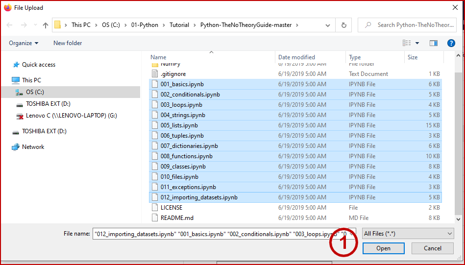
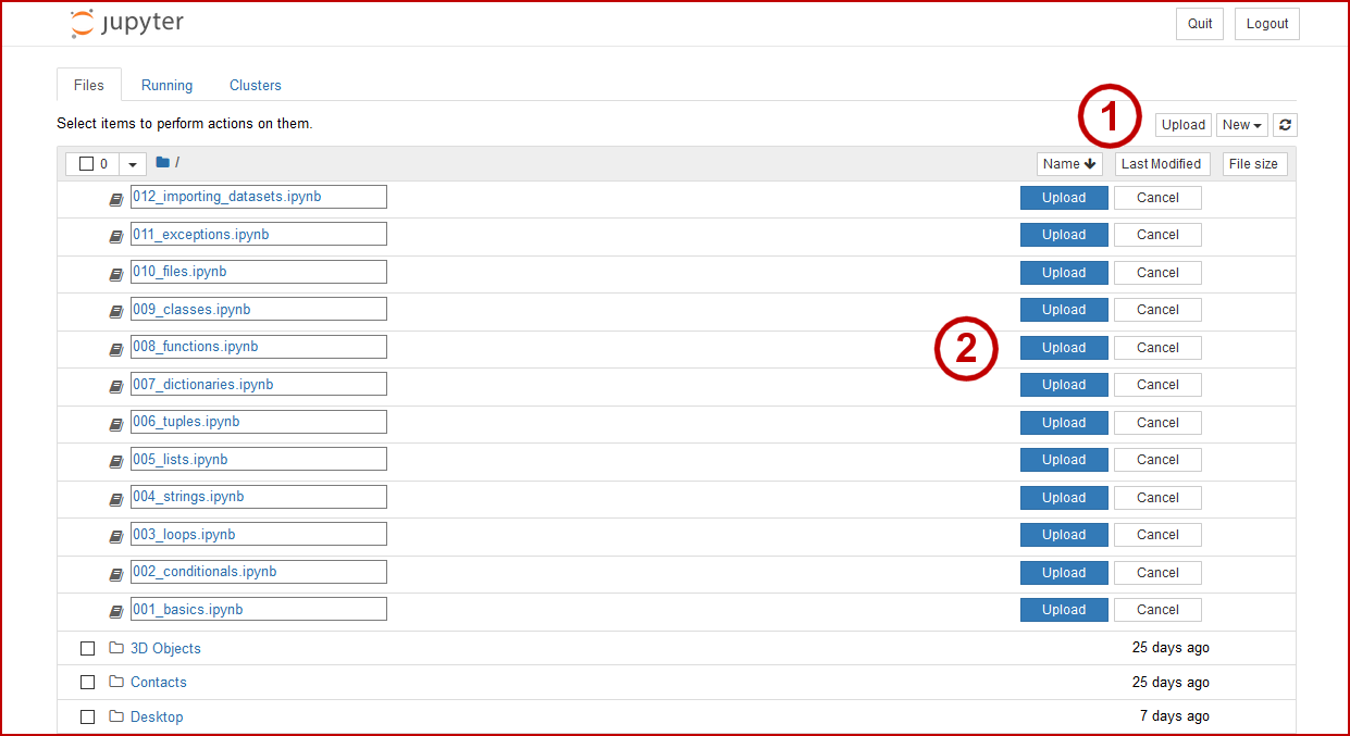
So, I have three choices. One, I could download and place my files into a directory under this default directory. However, that does not solve my initial problem. Two, I could download the files somewhere directly on my local machine, and then use the Upload option (1) in Figure 1 to move them into this default directory. To do so, I invoke the Upload button, which pulls up the Window Explorer for file uploads to which I navigate to the directory where I had just unzipped the files. I then highlight the unzipped files of interest (note they all have the *.ipynb extension):

When I enter the Open button (1) that selects all of the files and returns me to the main Jupyter screen, as shown in Figure 4:

As I pick Upload for each selected file (2), the file gets copied to the default directory and the Upload row is then deleted. I continue this process until all of the selected files have been copied.

But this approach still ends up storing my notebook files in a location not of my choosing. If I were only going to poke at this application on rare occasions, perhaps that is OK. Yet my plan is to use notebook files aggressively. So that leads me to the third option of changing the location of the default directory.

There is a two-step process to do so, First, we need to go to the default directory and look for the .jupyter sub-directory (note the preceding period!), which should appear as C:\Users\user\.jupyter. We bring up the command window here and enter and run at the prompt:

jupyter notebook --generate-config

This command creates a new file, C:\Users\user\.jupyter\jupyter_notebook_config.py, which is populated with the various command switches that govern the Jupyter Notebook’s behavior. In its initial condition, this file does not exist, and all settings reflect initial defaults. Once this file is generated, it is now possible to overwrite these default settings. BTW, this file can subsequently be deleted, in which case Jupyter Notebook reverts to its factory settings.

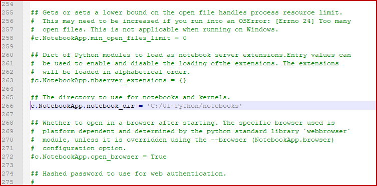
Open an editor for the jupyter_notebook_config.py and search for the following line in the file: #c.NotebookApp.notebook_dir = ''. It occurs about line 265 in the config file. Replace this text with your new desired starting root location for Jupyter. The entry should look like:

c.NotebookApp.notebook_dir = '/the/path/to/home/folder/'

When you make this update make sure you: 1) remove the # character at the beginning of the line and leave no space (the # designates the start of a comment line, and is thus not read at start-up time); 2) you use forward slashes in your path and do not use the tilde ~ character; and 3) you quote the file path in either matching single or double quotes. Figure 5 shows this modified config file for my own installation:

Once you complete the edits, save the file, and then re-start the Jupyter Notebook. Here we see the application now starts up at my preferred directory location:

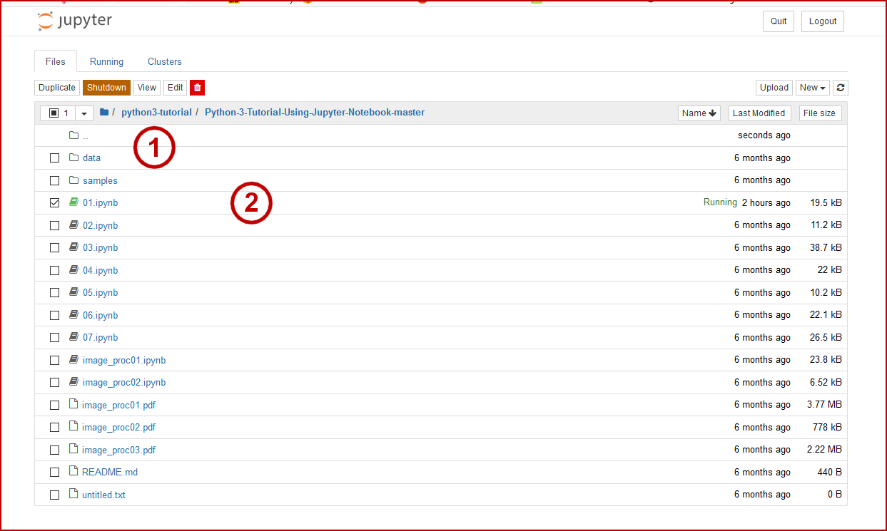
We can see we have a new directory structure (1). To open a Notebook page, we only need to double-click the entry (2) and we see that it is now running. Navigation through this tree file structure works as normally.

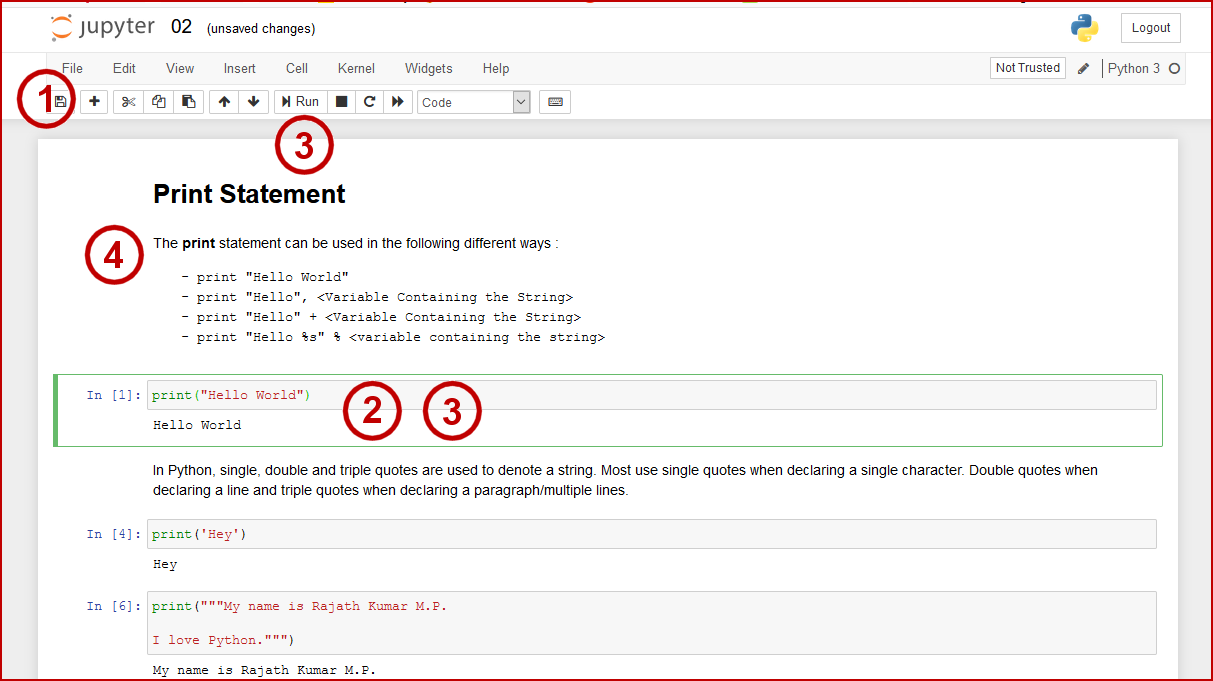
We will now select the second Notebook page on this list, 02.ipynb, and when we double-click it we get a new page in our browser with the new interactive page. Let’s explore some of the conventions of working with a Notebook page in Figure 7:

First, beside double-clicking, we may open and close Notebook pages using the old fashioned File option (1). Interactive areas of the Notebook page are shown as cells with the light gray background. The active interaction cell is bounded by the box with the margin highlight (2). To evaluate the cell in this active interactive we may either use the Run button or by using <shift>+<enter> when the cursor is in the active area (3). Also, the text on the page (4) may be entered or edited in the same way. We may either double-click or <shift>+<enter> when our cursor is in these text areas. Text entry occurs using a simple text formatting form called Markdown. We will be using Markdown aggressively throughout the rest of this series, and will have many occasions to describe its formatting and style options.

Like any document, existing Notebook pages can be loaded, modified, and saved again. This enables you to grab useful starting Notebooks on the Web, bring them into your own environment, modify them to reflect your own needs and circumstances, and then save them for later local use or for publishing to others. We can extend the active areas to include entire programs, with many complicated displays and activities possible in our Notebooks. This format is an excellent one for producing interactive dashboards and demos.

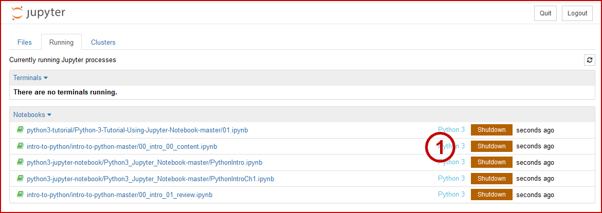
When we are done with our Notebook pages we may File → Close and Halt, Quit, which will stop the server and end all active pages, or use a Shutdown button for an individual page. As we shut individual pages, we are directed to a main screen that shows all of the Notebook pages currently active, which we may Shutdown directly (1) as Figure 8 indicates:

I encourage you to work through many of the examples provided in the three sources listed at the top of this article to gain a feel for Python syntax and the kinds of programming you can do with the language. The three sources at the beginning of this article proceed from simpler to more complicated within each source, and between sources, with the last example being the most comprehensive. The author of the last example suggests it takes about 90-120 hours to work through all of its examples [3]. Of course, simply browsing to gain a feel for the scope of the Python language can be done much quicker.

There are many online resources useful to Python programming. A simple Web search will turn up many Python learning scripts and examples. Here are some additional free ones I have found fairly useful:

• Interactive Python Tutorial from LearnPython.org
• Digital Ocean’s How to Code in Python3 Series
• Jupyter Notebook Tutorial from Google
• Jupyter Notebook Tutorial in Python from plotly (all tutorials in notebook form)
• Python Tutorial For Beginners – A Complete Guide
• Python3 Tutorial (see links in left-hand panel).

Endnotes:

This Will Also Test if Python is Working Correctly

You will recall from earlier installments in this Cooking with Python and KBpedia series that one design objective was to include a Python integrated development environment. The two leading IDE options within the data science community appear to be PyCharm and Spyder. Both are natively supported by our Anaconda package manager that we discussed in CWPK #9. My initial investigations indicated that PyCharm, the more popular option, was perhaps a bit more Mac oriented, maybe of more interest to coders and hackers, and perhaps less so from data scientists. PyCharm is one of a suite of well-regarded tools and environments from JetBrains. Spyder, on the other hand, draws its name from Scientific PYthon Development EnviRonment, has a cleaner look to my eye, and a paned layout I find a bit more intuitive.

Of course, the real worth of an IDE comes from its use, and some time of familiarity is always required before a judgment of adequacy can be made. Since my intuition steered me to Spyder, I chose to install it first. If it proves productive, there will be no need to veer from it. If I am not fully satisfied, I can always switch out to PyCharm or perhaps another alternative. This flexibility was a major reason for starting this Python process with the Anaconda distribution.

Since in the last installment we took the steps offered by the Anaconda Navigator GUI to install our Jupyter Notebook environment, let’s take the direct command-line approach for Spyder. Fortunately, we know that Spyder installation is already part of the Anaconda installation, so our task is much simplified to merely starting up and using the application.

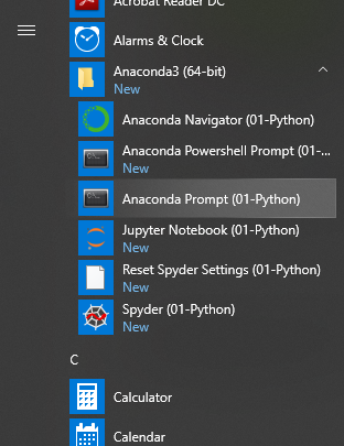
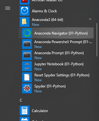
To begin our Spyder use, invoke the Windows Start menu and call up the Anaconda prompt option:

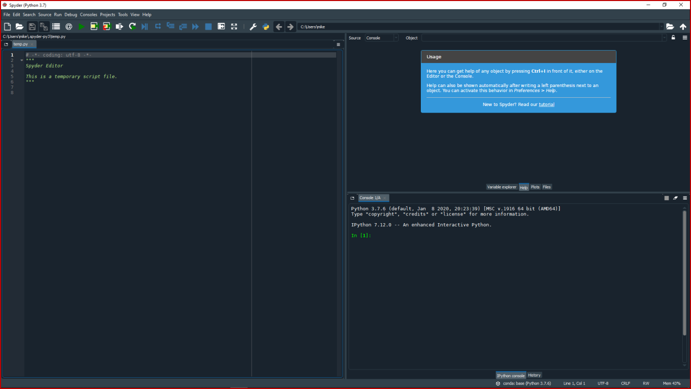
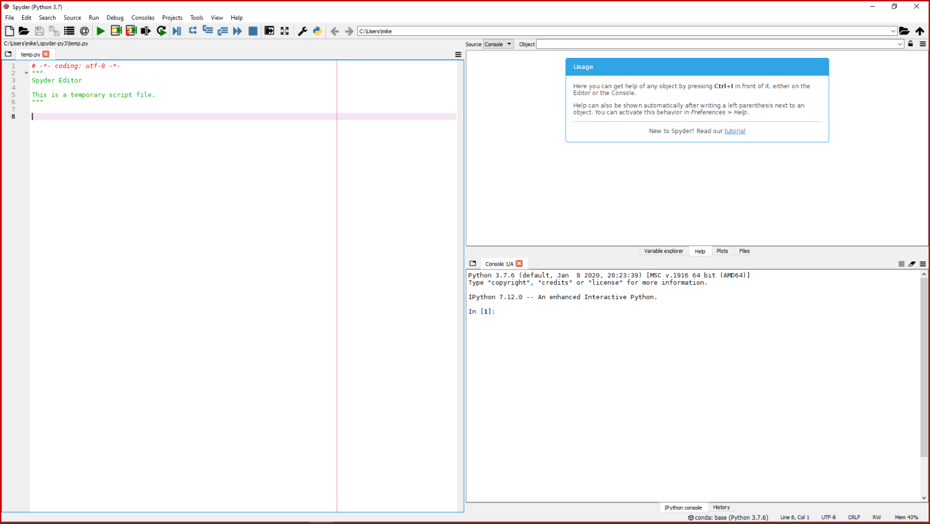
That calls up a command window, where we enter at the prompt, (base) C:\users\mike>spyder. (Your directory structure will differ.) That brings up the basic Spyder IDE, as shown in Figure 2:

However, if this is the first install, you might also get a popup window over this telling you that your Spyder version can be updated. It is important to remember that Python applications (of which both Anaconda and Spyder are examples) invoke many components to operate. These components are often shared by other applications and developed by third parties. Numerous releases of various component parts are constantly occurring throughout the Python ecosystem. One important role of package managers is to query for updates, alert you if components are out of date, and then enable you to update your packages. If you are an infrequent user of Python you will likely get update prompts for various components every time you use the system. Even daily use will see update notices quite frequently. If you see this notice that Spyder is out of date, Quit the program.

If you are only slightly out of date, you likely do not have concerning security holes or obsolete apps. You can proceed without updating. However, it is good practice to always respond to update requests. In this instance of the initial install of Spyder, we decide to install (and get rid of the annoying update screen at start-up). We go to File→ Quit on the Spyder screen. Since we started Spyder at the command line, we return to the command window. (If you had started up with the Anaconda Navigator option, you likely will need to go through the Anaconda prompt steps above to bring up the command window.)

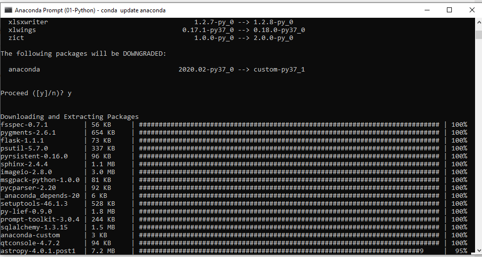
We can first update Spyder alone, and see if that leads to a clean start-up. At the command prompt enter (base) C:\users\mike>conda update spyder. The update facility will be invoked and you answer the prompts in the command window. When you re-start Spyder, however, you may again see the need to update screen. This likely notice is due to the fact that there are many dependencies across your entire Python environment. The better way to answer update prompts is by updating the entire environment. You invoke this more complete updata by entering at the command prompt: (base) C:\users\mike>conda update anaconda. (Your directory structure will differ.) Now, we see many packages needing to be updated and thus a more active update screen, as this Figure 3 example shows:

When you see the successful completion notice on the update, you can again start the Spyder IDE, now updated and missing the update notice screen.

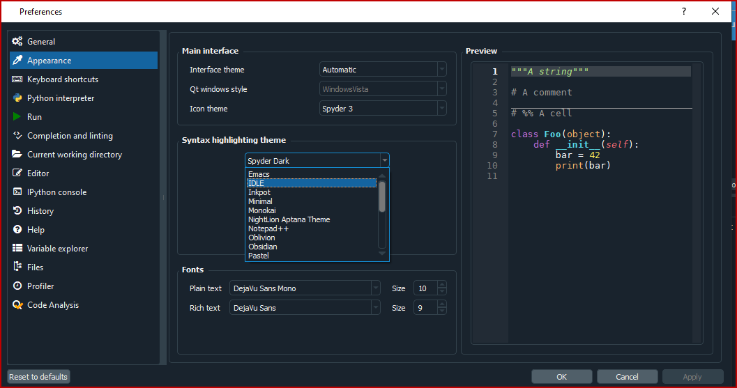
So, now we have an updated, current Spyder and Anaconda environment, with Spyder now invoked. By default at install time, Spyder is configured to use the currently popular dark theme, Spyder Dark. As a personal preference (and it is better for screen captures throughout our CWPK series) I like a lighter theme. To change the theme, we go to Tools → Preferences and then the Appearance option and see a listing of interface specifications:

We pick ‘IDLE’ since we know it to be a light one. (There are many loaded configurations you may test as well as create your own.) Once we select and hit the OK button, we are prompted if we want to re-start in order to use the new theme. We accept, and now see a different UI theme as shown by Figure 5:

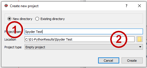
It is always a good idea to start any coding work with a project. We pick the Projects main menu option on main Spyder screen to do so:

We give our project any arbitrary name (1) and indicate the location for that file (2). It is a good idea to set up a known, separate directory location for your Python work. In my instance, I chose a new Results directory at the same level as my Python directory. By following this practice you will be better able to find prior work after absences away from the projects.

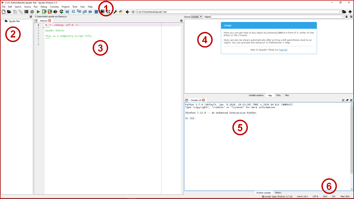
As you enter this project information, you may have been sharp-eyed and saw that a new pane has been added to the main Spyder screen at the left (2), as shown in Figure 7, which now gives us a chance to explain the panes and functions of the main Spyder IDE screen:

At the top of the main Spyder screen we have the main menu (1). It is a good idea to systematically move from menu item to item to see the functionality included in the Spyder IDE. Immediately below the main menu is the Toolbar. Again, you may mouse over each icon to get a tooltip of what functionality it represents. Note the icons are provided in groups, with debugging options provided in the middle, for example.

The leftmost pane (2) is the Projects pane. As your projects grow and you organize them, they are listed here in the traditional directory tree structure. Right-clicking on a project enables you to open, delete, use, etc., the project.

The main code editor is found in pane (3). Syntax highlighting and code completion assists of various natures may be invoked here, similar to any modern code editor. This is a window in which we will spend much time throughout this CWPK series. A general help area is provided in pane (4). You can pull up the general help, and get various prompts or assistance. In context, we will touch on some of these in later installments.

The console (5) is an interactive environment that shares the same iPython core with the Jupyter Notebook. Individual statements can be tested and run using REPL. Also, we can highlight code blocks in the editor (3) and they will run in this pane.

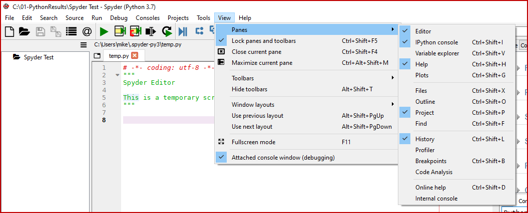
Notice that the horizontal pane separators may be moved. Each pane also has an upper right icon () that provides contextual options for that pane, including the standard options of Close or Undock. If you choose the Undock option, the pane becomes floating. To return it to its original position, chose the option to Dock. Note if you close a pane, you may open it up again via the View more Panes options. The ones we have active in this initial installation are shown in Figure 8 below.

You will notice that there are many possible panes in Figure 8 that are not shown as active. But, also notice we do have a History pane that is active that we have not yet discussed. When there are more panes selected for view for which there is not adequate screen space, multiples will appear in a given frame area as sub-tabs. If you look closely at the lower right of Figure 7 you will see this additional History tab (6). We also see some status information at the lower right in Figure 7 (6) that tells us what version of Python is presently loaded, line and character positions in the editor (3), etc.

If you only work occasionally with Python perhaps these options are enough to give you a fast configuration that meets your needs. Much of the stuff behind the scenes in Spyder, however, like other IDEs, is devoted to allow constant users to tweak the system to exactly how they want it.

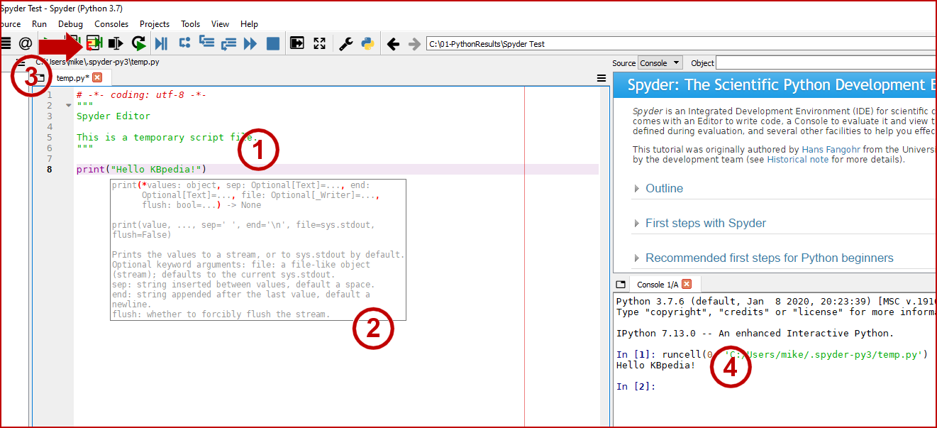
OK, so now we have gotten a bit familiar with Spyder and have configured it a bit to our liking. It is now time to write our first program. We will use Figure 9 to illustrate this process:

As with our previous lesson with Jupyter, we enter the statement print("Hello KBpedia!") (1). Note that as we enter statements, we get some autocomplete suggestions for our print statement. Once we have completed our statement, we can run this cell (3) from the Toolbar, which is another way of saying to run the current line, and its results appear in the console (4). Note we could just have easily entered the same print statement in (4) and gotten the same result evaluation. The difference, of course, is that statements entered into the editor are part of a conventional Python (*.py) source program as opposed to a single interactive statement. The same Toolbar where we ran the cell also allows us to run code blocks or the entire source program depending on the icon we select.

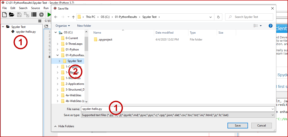
Now that we have completed our first file, it is time to save it, as shown by Figure 10:

The system allows us to save the code file anywhere, but again best practice is to enter the file name (1) under the same directory as our project location (2), which enables it to show (1) in the project pane. We then File → Quit to exit the program.

We will learn much about the Spyder IDE as we move forward. Here are some additional resources to learn about Spyder further:

• Spyder documentation
• How to Install the Python Spyder IDE and Run Scripts
• What is Python Spyder IDE and How to Use it?

This Will Also Test if Python is Working Correctly

In the previous installment in this Cooking with Python and KBpedia series, we installed Python via the Anaconda distro and package manager. The GUI portion of that package, Anaconda Navigator, was part of that install. In this current CWPK installment we will use Navigator to launch the Jupyter electronic notebook, and then write a simple program to demonstrate that our Python installation is installed properly and working. In the installment after this one, we will next install a Python IDE using the command line to demonstrate the second way we can interact with this package.

Though there are a variety of electronic notebooks that may work with Python, we have chosen Jupyter (nee iPython) because it is the oldest of Python notebooks, the most used, and the most capable. Like all of the packages we utilize in this CWPK series, the Jupyter notebook is open source. Two supplementary sources to this article are the Jupyter instructions on KDnuggets and or installing and testing the notebook.

We can launch Navigator either via the command line or directly from the application. We use the direct approach in this installment. We start Anaconda Navigator via the Windows Start button, and then expand the listing for Anaconda3 and pick Anaconda Navigator from the menu:

(Alternatively, you could pick ‘Anaconda Prompt’ from this menu and type the command anaconda-navigator.)

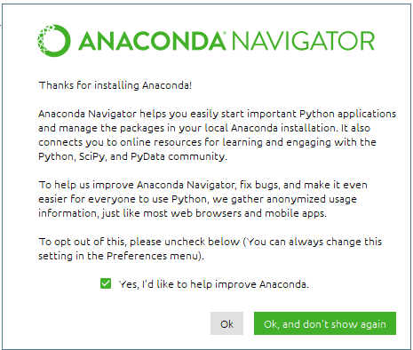
The first time you start Navigator, you will see a splash screen introducing the app and asking if you would be willing to share usage data. I picked Yes and then OK, and don’t show again:

We will thus not see this screen again at start-up.

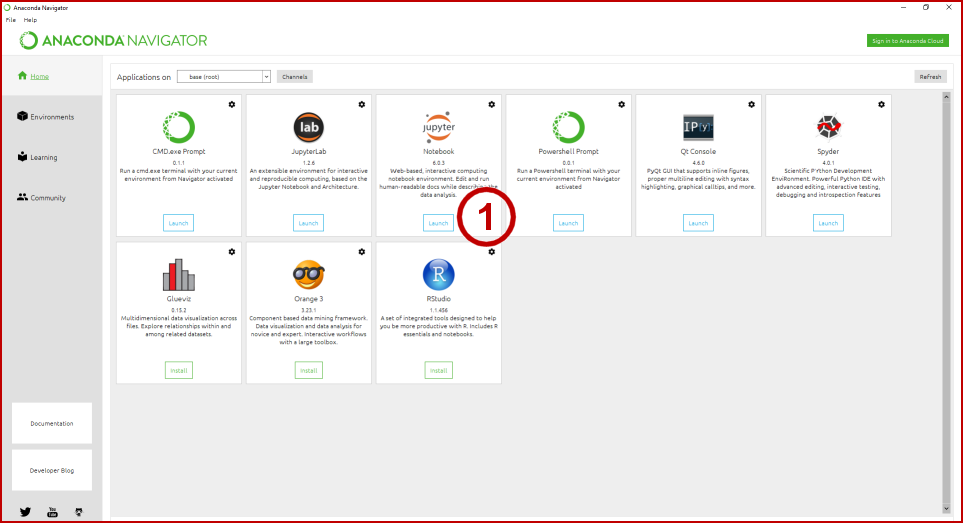
When invoked, we get this main (Home) launch screen for the Navigator:

We pick the Jupyter Notebook (1) from this list.

This launch then brings up a new Web page for the Jupyter Notebook application, as shown in Figure 4 below. (Note: if this step works, that means your Python installation from CWPK #9 is working properly.) Jupyter notebooks are presented as interactive HTML pages. This initial entry page is set by default to your user Web page. (We will later discuss how to set this to a different location.) The convention for Jupyter notebook files is *.ipynb. To start a new notebook, pick the dropdown menu labeled ‘New’ (1) at the upper right of this screen. You may then create a new Notebook with the Python version you installed:

Here is the new starting Notebook entry screen:

You may then rename your Notebook by clicking on a current name and editing it or by finding a name under File (3) in the top menu bar.

Now, in this simple example, we enter the statement (2) of print(“Hello KBpedia!”). That statement gets evaluated in real time (via the REPL loop previously mentioned) by pressing the Run button (1) into the result of ‘Hello KBpedia!’ [shown at bottom of (2)].

When done with this application, you exit by going to File at the upper left (3) and picking Close and Halt. That will return you to the main screen of Anaconda Navigator, where you may File → Quit to back you out of all programs. Should there be any open applications, you have the choice to close them as well at that time.

We will be working with Jupyter much throughout this CWPK series, and will thus have many opportunities to see other aspects of working with these notebooks. If you wish to learn more about notebooks, here are some resources:

• Jupyter notebook for beginners
• Jupyter notebook documentation
• Interactive notebook widgets and ipywidgets
• Best of Jupyter for Data Science
• JupyterLab is the next-generation user interface for Jupyter.

Trying to Take a Good First Step

We have spent a week and one-half setting the table and clearing our throats. It is now time to begin putting software into action. The complement to our KBpedia environment is the one for Python. We now switch gears to finding and installing a basic Python ‘starter package’ for this Cooking with Python and KBpedia series. We will approach this question from the standpoints of our local Windows 10 operating environment, the needs for KBpedia and its tools, and our desire to move into data science and machine learning applications.

Though I am an absolute newbie with regard to Python, I have been monitoring it for some years as a possible language to adopt. For quite a few years there was apparently a lengthy and difficult transition from Python 2 to Python 3. (As of this writing, the current version is Python 3.8.5.) Many of the issues we will address in coming installments deal with questions like encodings, management of CSV files, file I/O, and other topics that have apparently been much easier to handle with Python 3 (specifically since Python 3.6 and 3.7). Because of this transition, one may still find tutorials and online guidance offered in both Python 2 and 3 flavors. Fortunately, since all that we are developing in this series is new, we do not need to account for a legacy code base. We are thus free to not have to provide duplicate Python 2 and 3 routines. Please note, however, if you are using Python 2 locally that likely most of the routines offered during this series will not run without an upgrade.

Going back to the days of the LAMP stack on a Windows machine, which I did years ago with the XAMPP package, I am leery about installing languages and complicated stacks on Windows. Unlike Linux packages that can be installed with a single command, and easier methods on Macs as well, my impression is that Windows has never been a particularly friendly environment for installing natively non-Windows systems and applications. Though the official Python site has some impressive documentation and installation kits, including some nice kits from third parties, I decided going in that I wanted to use a more automated approach to handling Python and related package installation and dependencies. The dependencies portion is especially tricky since many data science applications with Python build on other packages, and getting them installed in the correct order with appropriate settings can be a real time waster.

My initial research suggested I wanted a data science focus for my Python installation with machine learning, of course. But, I also thought it might be a good idea to install an integrated development environment (IDE) to aid code completion, language lookup, and debugging. I also had become quite enamored with the REPL (read-eval-print-loop) capabilities in our Clojure work, which allows code snippets to be interpreted and run immediately, so I also was quite intrigued with adding an electronic notebook environment as well. My initial research suggested either the PyCharm or Spyder IDEs might be suitable for data science. I had already been following development with the Jupyter notebook (initially iPython) for quite some time and wanted to include that in my platform as well.

So, while I was beginning to zero in on a suite of Python-based tools, I had not worked directly with any of them. I therefore also wanted a Python package installer that was flexible enough to enable me to choose among alternative tools and switch them out if need be with relative ease. Who knows what kind of speedbumps I might encounter as we continue on the journey in this CWPK series? Prior experience with Eclipse and other IDEs warned me that component might especially be one that required some choice and flexibility.

There are a number of guides for installing Python locally that are quite good. One is geared around Jupyter and uses PyCharm as the IDE. I did not really like the lock-in on the IDE and also did not like the suggestion to immediately incorporate GitHub into the workflow. (GitHub is essential for anyone hoping to share code with others or develop an open-source package, but my target audience of the focused newbie may not require this step.) Other guides, however, for examples the ones from KDnuggets or DataCamp, kept pointing me to the open-source Anaconda installer package.

Anaconda is a package manager, an environment manager, and a Python distribution that particularly emphasizes data science applications. The environment enables one to quickly download more than 7,500 Python/R data science packages (so, it also supports incorporation of R; see CWPK #13), including the essential ones of machine learning in scikit-learn, TensorFlow, and Theano, plus the data analysis tools of Dask, NumPy, pandas, and Numba. Multiple data visualization packages of Matplotlib, Bokeh, Datashader, and Holoviews can also be managed. Anaconda enables one to manage libraries and their dependencies on Windows, MacOS and Linux using the Conda package manager. Conda complements the standard pip Python package manager. More than 20 million users worldwide use the Individual Edition version of Anaconda.

The final factor that convinced me to use Anaconda was its Navigator graphical user interface that enables one to launch applications or manage packages. Navigator showed me a way to easily choose Jupyter, PyCharm or Spyder, three of the big options at the center of this work, among many other package choices down the road. Thus, while I may prefer working directly in an editor via an IDE when writing programs, having the option to manage apps and dependencies in a GUI is really attractive.

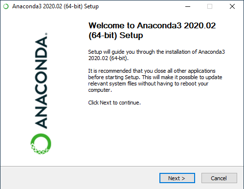
Installation of Anaconda is a breeze, though I do add one important wrinkle to the fully automated path.[1] Begin by going to the Anaconda Individual Edition download page and pick Download:

When presented with the alternative approach, choose it. While it is nice to have the Anaconda GUI available for some tasks, we also want to work with Python at the command line without needing to invoke Anaconda. The alternate path approach writes the appropriate path information to the Windows environment variables, meaning we can invoke Python and related applications from any location on our local machine.

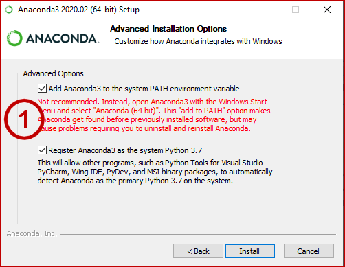
Your first actual install screen will ask about Advanced Options. Make sure and pick the Add Anaconda3 to the system PATH environment variable. When you do, you will get a red font notice telling you this option is not recommended. Proceed with it anyway by picking Install:

You will then have the choice to install as a single user or for the entire machine. In my case, since it is a dedicated computer not on a business network, I use the entire machine option. Your local circumstance or IT department may mandate the single user option.

You should pause at this point and think through what you want your directory structure to be. You can accept placing all files in standard install locations (assuming a C: drive) of C:\Users\mike\anaconda3 if you set it up for you as a single user, or C:\ProgramData\Anaconda3 if you selected to install for all users. However, I find it useful to set up my own directory structures and be able to modify and expand at will. A Python installation with Anaconda will take substantial space, and you may be setting configurations for many different apps as well as projects other than KBpedia or derivatives. For security purposes, we also want to keep our use of Python somewhat fenced and unable to reach the root. (We’ll discuss this again in CWPK #15.) Here is how I am setting up my directory structure:

|-- PythonProject                         # Set up a 'master' directory for all of your Python work; name as you wish 
     |-- Python                           # Create a 'Python' (upper or lower) directory under this root
           |-- [Anaconda3 distribution]   # Direct your Anaconda install to this location
     |-- TBA
           |-- TBA                        # We'll add to this directory structure as we move on
     |-- TBA
           |-- TBA

The entire install process is automated by following the instructions on each screen. During the actual install process you may click the Details button and watch progress as it proceeds file by file. The longest step is setting up the package cache. Overall the installation takes a few minutes. Please be patient. At the conclusion of the installation and feedback to the screen, proceeding through all steps as presented, we conclude by clicking on Finish.

To check to see if the install proceeded properly, call up a command prompt (Powershell or cmd at the Windows Run option), and see if you get version information for these two commands:

conda --version
python --version

If you get version information echoed to the screen, you are fine. If these commands do not work, see the ‘Add Anaconda to Path (Optional)’ section in DataCamp.

If you have Windows issues, you can inspect the general Python Windows use guide or look into these possible issues after install.

For additional information about Anaconda, see the quick start user guide or the getting started tutorial (requires registry).

The ease of installation and package management with Anaconda does come at the cost of some bloat, as well as higher memory requirements for what gets loaded at start up. For the former problem, it is possible to replace Anaconda at a later date with Miniconda and conda, especially as your environment has stabilized and you have less frequent need for Navigator package manager. As for memory management, if your machine is only marginally capable, you may want to look into these scripts or these other scripts.

Endnotes:

A Survey of the Upper Ontology, Full Knowledge Graph, and Typology Design

Now that we have become a bit familiar with Protégé and have our local file structure set, let’s conduct a brief survey of the main components of the KBpedia structure. We’ll be using Protégé exclusively during this installment of the Cooking with Python and KBpedia series.

Start up Protégé as we discussed in CWPK #6. This time, however, use File → Open . . . and navigate to your KBpedia directory, and then the ‘owl’ subdirectory and the kko-demo.n3 file, highlight it, and pick Open. You should see a screen similar to Figure 1 after going to the Classes tab and expanding parts of the tree to expose some of the structure under the SuperTypes or Generals branch:

You will note (1) that sub-items under each leaf are listed in alphabetical order. If you recall, however, we have organized the upper structure of KBpedia according to Charles Peirce‘s universal categories of Firstness (1ns), Secondness (2ns), and Thirdness (3ns). Roughly speaking, these categories correspond to qualities or possibilities (1ns), actuals or particulars (2ns), or generals (3ns).[1] Though we have provided metadata as to which of these three categories is assigned to each KBpedia reference concept (RC), we can not see these assignments in this listing. The purpose of the kko-demo.n3 file is to make these assignments explicit via the Protégé interface. We do this by assigning a prefLabel (preferred label) to each RC prefixed with its universal category number. (This change makes this particular file inoperable, but it does serve a didactic purpose to better understand KBpedia’s upper structure.)

To see this assignment, we need to change the basis for how Protégé renders its labels. To do so, proceed to the File → Preferences . . . and then the Renderer tab as shown in Figure 2. Depending on how your system is configured, you may need to both select the ‘Render by annotation property (e.g., rdfs:label, skos:prefLabel’ radio button and use the Configure . . . button to instruct what property to use for this label. If your Configure . . . popup screen does not show the http://www.w3c.org/2004/02/skos/core#prefLabel option in the top position, either move it to be the top option or choose the Add Annotation button at the upper left of the dialog; you will find the skos:prefLabel under the rdfs:label entry. Note, via these steps you can configure Protégé to display a variety of label choices.

With this change made, we then expand out the Class hierarchy tree to the same point. Only now, we see labels prefixed with the universal category numbers, which also acts to re-order the entries, as Figure 3 shows:

With this labeling now operating, we can navigate to the OWLViz tab, as we begin to show in Figure 4. (If OWLViz is not active in your installation, please refer to the OWLViz plug-in page and follow the installation instructions to activate that plug-in and get it set-up properly.) Since we want to see the layout structure of the Generals node where the KBpedia typologies reside, we first navigate to that node in the Class hierarchy tree (1). By picking the rightmost button in the display pane header (2) we can configure the depth to be shown in this display (3). We pick ‘5’ levels to track, resulting in the display below:

With this level of expansion, there are too many items to see within the available pane. We need to scroll to see the full extent of the structure. However, if we want a more comprehensive view, we can also export the entire image to file.

We do so, as Figure 5 indicates, by picking the next to rightmost pane header button (1) and then picking to display only the asserted items (2). When we pick Next we are given a dialog that enables us to set the image format type and to possibly scale the image. We accept the defaults, and then proceed to save our image with a name we prefer to our desired disk location.

This now produces for us a full rendering of the KKO ‘Generals’ structure, as shown in Figure 6:

Note we would have gotten the entire KKO structure if we had chosen the owl:Thing node as our starting location for the OWLViz graph rendering as opposed to ‘Generals’.

It is worth your time to study this KKO structure closely. The ‘Generals’ branch, in particular, is where all of KBpedia’s typologies reside (and therefore the great bulk of the RCs in KBpedia). Most every node in KKO under the Generals branch is itself the root node for a corresponding typology.

Though there are nearly 70 typologies in the KBpedia system, about 30 of them host the largest number of RCs and also have disjoint (non-overlapping) assertions between them. Here are the 30 or so core typologies organized in the KKO graph, with some upper typologies that cluster them:

Once you have gained a feel for the upper KKO structure, it is useful to see how that organizes the entire content across the full KBpedia knowledge graph. So, once you are done inspecting KKO, go back to the File → Open recent . . . dialog, pick the ‘ . . . \target\kbpedia_reference_concepts.n3‘ full ontology file (the one we earlier inspected in CWPK #6) and answer Yes to the ‘Do you want to open the ontology in the current window?’ dialog. Also agree to let the shared items remain in the workspace.

With the familiarity gained from our inspection of the KKO, it becomes a bit easier to see how the detailed RCs fit within this overall KKO upper structure. Note, however, that we no longer have the universal category prefixes that our non-working kko-demo.n3 view gave us. Again, spend some time continuing to get familiar with the scope of reference concepts in KBpedia including use of the search function as explained in CWPK #6.

Another step we can take is to review the individual typologies in isolation. If we return to the File → Open dialog we can navigate to the ‘typologies’ directory within our chosen KBpedia file structure. Let’s scroll through that list and then select one, say, Facilities-typology.n3. We will again in the dialog accept to open the ontology in the current window by choosing Yes. The facilities typology will then load, presenting to us the opening Protégé screen with most of the metadata blank. Then, select the Classes tab and begin expanding the Classes hierarchy tree as shown in Figure 7:

Remember from our brief build overview in CWPK #2 that one of the last steps in the build process was to create these typology files. Thus, while the expandable Class hierarchy pane (1) shows the expected tree structure, the annotations pane (2) is empty and the descriptions pane (3) only shows the direct subClassOf linkages. That is because these typology ontologies are an extraction from the full knowledge graph and are not meant to be usable on their own.

In this manner you can inspect any and all of the KBpedia typologies that may be of interest to you in isolation. Though many RCs have more than one typology assignment, this isolated view removes that complexity. These isolated typology views are particularly helpful when adding a new typology to the system or when trying to understand the scope of a given typology.

Endnotes: