Posted:August 26, 2020

Using the Direct Approach with Owlready2
In this installment of the Cooking with Python and KBpedia series, we explore ways to directly search knowledge graph text from within the owlready2 API. We first introduced this topic in CWPK #19; we explain further some of the nuances here.

Recall that owlready2 uses its own local datastore, SQLite, for storing its knowledge graphs. Besides the search functionality added in Owlready2, we will also be taking advantage of the full-text search (FTS) functionality within SQLite.

Load Full Knowledge Graph

To get started, we again load our working knowledge graph. In this instance we will use the full KBpedia knowledge graph, kbpedia_reference_concepts.owl, because it has a richer set of contents.

Which environment? The specific load routine you should choose below depends on whether you are using the online MyBinder service (the ‘raw’ version) or local files. The example below is based on using local files (though replace with your own local directory specification). If loading from MyBinder, use this address for kbpedia_reference_concepts.owl
main = 'C:/1-PythonProjects/kbpedia/sandbox/kbpedia_reference_concepts.owl'
# main = 'https://raw.githubusercontent.com/Cognonto/CWPK/master/sandbox/builds/ontologies/kbpedia_reference_concepts.owl'
skos_file = 'http://www.w3.org/2004/02/skos/core' 
kko_file = 'C:/1-PythonProjects/owlready2/kg/kko.owl'
# kko_file = 'https://raw.githubusercontent.com/Cognonto/CWPK/master/sandbox/builds/ontologies/kko.owl'

from owlready2 import *
world = World()
kb = world.get_ontology(main).load()
rc = kb.get_namespace('http://kbpedia.org/kko/rc/')

skos = world.get_ontology(skos_file).load()
kb.imported_ontologies.append(skos)

kko = world.get_ontology(kko_file).load()
kb.imported_ontologies.append(kko)

To execute the load, pick shift+enter to execute the cell contents, or pick Run from the main menu.

Besides changing our absolute file input, note we have added another scoping assignment world to our load. world is a reserved keyword in Owlready2 that encompasses the SQLite storage space used by Owlready2. Note we assign all of our ontologies (knowledge graphs) to this namespace so that we may invoke some of the FTS functionality later in this installment.

Basic Search Functions

As the owlready2 documentation explains, it contains some pre-loaded search capabilities that can be performed with the .search() query method. This method can accept one or several keyword arguments:

  • iri – for searching entities by their full IRIs
  • type – for searching instances for a given class
  • subclass_of – for searching subclasses of a given class
  • is_a – for searching both instances and subclasses of a given class, or object, data or annotation property name.

Special arguments that may be added to these arguments are:

  • _use_str_as_loc_str – whether to treats plain Python strings as strings in any language (default is True)
  • _case_sensitive – whether to take lower/upper case into consideration (default is True).

Our search queries may accept quoted phrases and prefix or suffix wildcards (*). Let’s look at some examples combining these arguments and methods. Our first one is similar to what we presented in CWPK #19:

world.search(iri = "*luggage*")
[]

Notice our result here is an empty set, in other words, no matches. Yet we know there are IRIs in KBpedia that include the term ‘luggage’. We suspect the reason for not seeing a match is that the term might start with upper case in our IRIs. We will set the case sensitivity argument to false and try again:

world.search(iri = "*luggage*", _case_sensitive = False)

Great! We are now seeing the results we expected.

Note in the query above that we used the wildcard (*) to allow for either prefix or suffix matches. As you can see from the results above, most of the search references match the interior part of the IRI string.

The iri argument takes a search string as its assignment. The other three keyword assignments noted above take an object name, as this next example shows:

world.search(subclass_of=rc.Mammal)

We get a tremendous number of matches on this query, so much so that I cleared away the current cell output (via Cell → Current Outputs → Clear, when highlighting this cell). To winnow this results set further, we can combine search terms as the next example shows. We will add to our initial search a string search in the IRIs for which prior results might represent ‘Bats’:

world.search(subclass_of=rc.Mammal, iri = "*Bat*")
[rc.Bat-Mammal, rc.SacWingedBat, rc.BulldogBat, rc.FreeTailedBat, rc.HorseshoeBat, rc.SchreibersBat, rc.WesternSuckerFootedBat, rc.AfricanLongFingeredBat, rc.AfricanYellowBat, rc.AllensYellowBat, rc.AsianPartiColoredBat, rc.DaubentonsBat, rc.EasternRedBat, rc.GreatEveningBat, rc.GreaterTubeNosedBat, rc.GreyLongEaredBat, rc.HawaiianHoaryBat, rc.KobayashisBat, rc.LesserYellowBat, rc.LittleTubeNosedBat, rc.NewGuineaBigEaredBat, rc.NewZealandLongTailedBat, rc.NorthernLongEaredBat, rc.PallidBat, rc.SilverHairedBat, rc.SpottedBat, rc.AfricanSheathTailedBat, rc.AmazonianSacWingedBat, rc.BeccarisSheathTailedBat, rc.ChestnutSacWingedBat, rc.DarkSheathTailedBat, rc.EcuadorianSacWingedBat, rc.EgyptianTombBat, rc.FrostedSacWingedBat, rc.GraySacWingedBat, rc.GreaterSacWingedBat, rc.GreaterSheathTailedBat, rc.GreenhallsDogFacedBat, rc.HamiltonsTombBat, rc.HildegardesTombBat, rc.LargeEaredSheath-TailedBat, rc.LesserSacWingedBat, rc.LesserSheathTailedBat, rc.MauritianTombBat, rc.NorthernGhostBat, rc.PacificSheathTailedBat, rc.PelsPouchedBat, rc.PeterssSheathTailedBat, rc.ProboscisBat, rc.RaffraysSheathTailedBat, rc.SerisSheathtailBat, rc.SeychellesSheathTailedBat, rc.ShaggyBat, rc.ShortEaredBat, rc.SmallAsianSheathTailedBat, rc.TheobaldsTombBat, rc.ThomassSacWingedBat, rc.TroughtonsPouchedBat, rc.AntilleanFruitEatingBat, rc.BidentateYellowEaredBat, rc.BigEaredWoolyBat, rc.CommonVampireBat, rc.HairyLeggedVampireBat, rc.HonduranWhiteBat, rc.LesserLongNosedBat, rc.MexicanLongNosedBat, rc.SpectralBat, rc.VampireBat, rc.WhiteWingedVampireBat, rc.GreaterBulldogBat, rc.LesserBulldogBat, rc.BigCrestedMastiffBat, rc.BigFreeTailedBat, rc.BlackBonnetedBat, rc.BroadEaredBat, rc.EuropeanFreeTailedBat, rc.GallaghersFreeTailedBat, rc.IncanLittleMastiffBat, rc.LittleGoblinBat, rc.MexicanFreeTailedBat, rc.NatalFreeTailedBat, rc.PetersWrinkleLippedBat, rc.SumatranMastiffBat, rc.WroughtonsFreeTailedBat, rc.LesserFalseVampireBat, rc.YellowWingedBat, rc.BigNakedBackedBat, rc.ParnellsMustachedBat, rc.NewZealandGreaterShortTailedBat, rc.NewZealandLesserShortTailedBat, rc.BatesSlitFacedBat, rc.LargeSlitFacedBat, rc.DayakFruitBat, rc.LittleMarianaFruitBat, rc.LivingstonesFruitBat, rc.MarianaFruitBat, rc.PetersDiskWingedBat, rc.Bat-earedFox, rc.AboBat, rc.JapaneseHouseBat, rc.BigBrownBat, rc.NorthernBat, rc.GrayBat, rc.GreaterMouseEaredBat, rc.HodgsonsBat, rc.IkonnikovsBat, rc.IndianaBat, rc.LittleBrownBat, rc.NatterersBat, rc.GreaterNoctuleBat, rc.VirginiaBigEaredBat, rc.GreaterHorseshoeBat, rc.LamottesRoundleafBat, rc.LesserHorseshoeBat, rc.MalayanRoundleafBat, rc.VietnamLeafNosedBat, rc.PersianTridentBat, rc.BondaMastiffBat, rc.VelvetyFreeTailedBat, rc.WesternMastiffBat, rc.MexicanFunnelEaredBat, rc.AndersensFruitEatingBat, rc.JamaicanFruitBat]

Again, we get a large number of results. There are clearly many mammals and bats within the KBpedia reference graph!

Per the listing above, there are a number of these pre-configured search arguments directly available through Owlready2.

We can also instruct the FTS system in SQLite that we want to index still additional fields. Since we are interested in a term we know occurs in KBpedia’s annotations relating some reference concepts to the UN standard products and services codes (UNSPSC) we try that search directly:

world.search(entered = "*UNSPSC*")
[]

Hmm, this tells us there are no results. We must be missing an indexed field. So, let’s instruct the system to add indexing to the definition property where we suspect the reference may occur. We do so using the .append method to add a new field for our RC definitions (skos.definition) to the available FTS index structure:

world.full_text_search_properties.append(skos.definition)

Since this is just a simple assignment, when we Run the cell we get no results output.

However, that assignment now allows us to invoke the internal FTS (full-text search) argument:

world.search(definition = FTS("UNSPSC*"))

If you get an ‘operational error’ that means you did not Run the .append instruction above.

Like some of the other listings, this command results in a very large number of results, a couple of which are warnings we can ignore, so we again Clear the Cell. We can get a smaller listing with another keyword search, this time for the wildcarded ‘gear*’ search:

world.search(definition = FTS("gear*"))
[rc.undercarriage, rc.number-of-forward-gears, rc.vehicle-transmission, rc.AutomaticTransmission, rc.BearingBushingWheelGear, rc.BevelGear, rc.Bicycle-MultiGear, rc.BoeingAH-64Apache, rc.BugattiVeyron, rc.ChildrensWebSite, rc.CombatSportsEvent, rc.Commercialism, rc.CyclingClothing, rc.Device-FunctionallyDefective, rc.FirstNorthAmericansNovels, rc.Fishery, rc.FreeDiving, rc.Game-EquipmentSet, rc.Gear, rc.GearManufacturingMachine, rc.Gearing-Mechanical, rc.GearlessElectricDrive, rc.Goggles, rc.Harness-Animal, rc.Helmet, rc.IlyushinIl-30, rc.LandingGearAssembly, rc.MachineProtocol, rc.Mechanism-Technology, rc.Overdrive-Mechanics, rc.PinionGear, rc.ProtectiveEquipment-Human, rc.ProtectiveGear, rc.ScubaGear, rc.ScubaSnorkelingGear, rc.ShockAndAwe-MilitaryTactic, rc.Supercharger, rc.TeacherTrainingProgram, rc.Trek, rc.Wheel, rc.WildernessBackpacking, rc.WormGear]

Notice in this search that we are able to use the suffix wildcard () character. However, unlike the standard OWLready2 search, we are not able to use a wildcard () prefix search.

Since we have added a new indexed search table to our system, we may want to retain this capability. So, we decide to save the entire graph to the database, as the last example shows:

world.set_backend(filename = 'cwpk-23-text-searching-kbpedia.db', exclusive = False)

This now means our database has been saved persistently to disk.

If you run this multiple times you may get an operational error since you have already set the backend filename.

We can then .save() our work and exit the notebook.

world.save()

Additional Documentation

Here is additional information on the system’s text searching capabilities:

NOTE: This article is part of the Cooking with Python and KBpedia series. See the CWPK listing for other articles in the series. KBpedia has its own Web site.
NOTE: This CWPK installment is available both as an online interactive file or as a direct download to use locally. Make sure and pick the correct installment number. For the online interactive option, pick the *.ipynb file. It may take a bit of time for the interactive option to load.
I am at best an amateur with Python. There are likely more efficient methods for coding these steps than what I provide. I encourage you to experiment — which is part of the fun of Python — and to notify me should you make improvements.

Posted by AI3's author, Mike Bergman Posted on August 26, 2020 at 2:07 pm in CWPK, KBpedia, Semantic Web Tools | Comments (0)
The URI link reference to this post is: https://www.mkbergman.com/2356/cwpk-23-text-searching-kbpedia/
The URI to trackback this post is: https://www.mkbergman.com/2356/cwpk-23-text-searching-kbpedia/trackback/
Posted:August 25, 2020

Some More Basics About Ontology Components

We began looking at managing classes in our last installment of the Cooking with Python and KBpedia series. We continue on that quest in this current installment, expanding our basic commands for instances, data and object properties, annotations, property relations, and operators. We do not probe all available methods, but emphasize those most often encountered. See the Additional Documentation sources at the end of this installment to get further information.

This present installment, plus the prior one, will complete our initial introduction into the ontology management functions available in owlready2. From here we next introduce some of the more advanced features in this API.

To interact with this installment on Jupyter Notebook, we will be using the smaller KKO (Kbpedia Knowledge Ontology), kko.owl, because it is a bit easier to inspect and manipulate.

General Load Method

Note we are continuing to consolidate our initial load statements into a single routine, which we will often use to begin subsequent installments. We also continue to follow the best practice of using logical names to refer to absolute file addresses.

Which environment? The specific load routine you should choose below depends on whether you are using the online MyBinder service (the ‘raw’ version) or local files. The example below is based on using local files (though replace with your own local directory specification). If loading from MyBinder, use this address for kko.owl


main = 'C:/1-PythonProjects/kbpedia/sandbox/kko.owl'

# main = 'https://raw.githubusercontent.com/Cognonto/CWPK/master/sandbox/builds/ontologies/kko.owl'

skos_file = 'http://www.w3.org/2004/02/skos/core'
from owlready2 import * kko = get_ontology(main).load() skos = get_ontology(skos_file).load() kko.imported_ontologies.append(skos)

Having executed these methods with the shift+enter or Run command from the main menu, we can now do a quick inspection to see if everything has loaded properly. We again use a listing of subclasses of the Products class:

list(kko.Products.subclasses())
[kko.PrimarySectorProduct,
kko.SecondarySectorProduct,
kko.TertiarySectorService]

Instances

Instance assignments work similarly to classes, except we must relate the new instance to its parent class. In this example, we are adding a camera instance to our SecondarySectorProduct class, itself a subclass of Products. We also add a print statement to confirm our assignment worked OK:

camera = kko.SecondarySectorProduct("camera")
print(camera.name)
camera

Like for classes, there are multiple methods for creating a new instance. Here is another form:

computer = kko.SecondarySectorProduct("computer", 
    namespace = kko)

The .instances() class method can be used to iterate through all Instances of a class (including its subclasses). It returns a generator:

for i in kko.SecondarySectorProduct.instances(): print(i)
kko.camera
kko.computer

Go ahead and substitute ‘Products‘ for the class name above to verify it also works on subclasses.

As we learned in the last installment, we can also delete the instance and all of its internal references:

destroy_entity(computer)

Data and Object Properties

Recall that the basic statement (assertion) in RDF, the base language of our ontologies, is a ‘triple‘. The triple has the form of subject – property – object (or s-p-o; also, predicate or relation is a synonym for property). Data and object properties may be inferred over in a W3C ontology. Object properties require a defined and named object (instance or class) as its object. Data properties require a datatype as its object, including strings. Annotation properties (see below) also take strings or URIs as their object, but can not be inferred over.

One creates properties in a similar manner to classes. In this example, we are creating the has_color sub-property of the qualities property, itself a sub-property of an ObjectProperty:

with kko:
    class has_color(kko.qualities): pass

You will note in this example that we used the underscore character to separate our names to make the property name more readable. Actually, in KKO (and KBpedia) our preferred convention is to use CamelCase with classes initially capitalized, and properties initially lower case. We do not use the underscore. What is important to note here, however, is that these are only best-practice conventions. There is no absolute requirement for classes, individuals or properties to assume a particular naming form.

To see that our new property has been properly added, we can do our standard list method:

list(kko.properties())

We can delete properties and all internal references with the destroy_entity method. Further, we can make domain and range assignments and other specifications of properties, some addressed below, the others covered in the Additional Documentation section.

Annotations

As noted, annotations are one of the property types where the objects are names or strings or link addresses (IRIs), but over which no reasoning may occur. Annotations provide the labels, definitions, comments, and pointers to the actual objects in the system. We can assign values in a straightforward manner to annotations (in this case, altLabel):

computer.altLabel = ["Mike's computer","PC", "workstation"]

We can confirm the properties assigned to the computer instance with the get_properties method:

kko.computer.get_properties()
{core.altLabel}

We can also see the actual altLabels were properly assigned:

print(kko.computer.altLabel)
["Mike's computer", 'PC', 'workstation']

You will note that the first label in the example above is shown with double-quotes in order to properly account for the single quote in the label for possession.

Like all properties in the system we can get a listing of the properties and classes that have assigned values for that property with this form of .get_relations method:

list(skos.altLabel.get_relations())

Indirect Relations

There is a special method in Owlready2 called ‘INDIRECT_‘. Invoking this brings up results for:

  • transitive, symmetric and reflexive properties
  • property inheritance (i.e., subproperties)
  • classes of an individual
  • class inheritance (i.e., parent classes), and
  • equivalences (equivalent classes, sameAs individuals).

Here is an example:

print(computer.INDIRECT_altLabel)
["Mike's computer", 'workstation', 'PC']

Property Restrictions

Owlready2 enables us to also place restrictions on our classes through a special type of class constructed by the system.

  • some – Property.some(Range_Class)
  • only – Property.only(Range_Class)
  • min – Property.min(cardinality, Range_Class)
  • max – Property.max(cardinality, Range_Class)
  • exactly – Property.exactly(cardinality, Range_Class)
  • value – Property.value(Range_Individual / Literal value)
  • has_self – Property.has_self(Boolean value).

These are the same names and understandings as is used by the Protégé ontology IDE (see CWPK #5). See further Additional Documentation for details.

Operators

Owlready2 provides three logical operators between classes (including class constructs and restrictions):

  • ‘&’ – And operator (intersection). For example: Class1 & Class2. It can also be written: And([Class1, Class2])
  • ‘|’ – Or operator (union). For example: Class1 | Class2. It can also be written: Or([Class1, Class2])
  • Not() – Not operator (negation or complement). For example: Not(Class1).

Save and Exit

When we are finished with our tests, we can File → Save and Checkpoint, Rename our output file, or specify it at the command line (substituting your own local preferences):

kko.save(file = "C:/1-PythonProjects/kbpedia/sandbox/kko-test.owl", format = "rdfxml")

Additional Documentation

Here are links to other owlready2 documentation:

NOTE: This article is part of the Cooking with Python and KBpedia series. See the CWPK listing for other articles in the series. KBpedia has its own Web site.
NOTE: This CWPK installment is available both as an online interactive file or as a direct download to use locally. Make sure and pick the correct installment number. For the online interactive option, pick the *.ipynb file. It may take a bit of time for the interactive option to load.
I am at best an amateur with Python. There are likely more efficient methods for coding these steps than what I provide. I encourage you to experiment — which is part of the fun of Python — and to notify me should you make improvements.

Posted by AI3's author, Mike Bergman Posted on August 25, 2020 at 11:19 am in CWPK, KBpedia, Semantic Web Tools | Comments (0)
The URI link reference to this post is: https://www.mkbergman.com/2355/cwpk-22-basic-knowledge-graph-management-ii/
The URI to trackback this post is: https://www.mkbergman.com/2355/cwpk-22-basic-knowledge-graph-management-ii/trackback/
Posted:August 24, 2020

Let’s Recap Some Useful Python Guidance

All installments in this Cooking with Python and KBpedia series have been prepared and written in order, except for this one. I began collecting tips about how best to use the cowpoke package and Python about the time this installment occurred in sequence in the series. I have accumulated use tips up through CWPK #60, and now am reaching back to complete this narrative.

Since we are principally working through the interactive medium of Jupyter Notebook for the rest of this CWPK series, I begin by addressing some Notebook use tips. Most of the suggestions, however, deal with using the Python language directly. I have split that section up into numerous sub-topics.

An interesting aspect of using owlready2 as our API to OWL is its design decision to align classes within RDF and OWL to the class concept in Python. My intuition (and the results as we proceed) tells me that was the correct design decision, since it affords using Python directly against the API. However, it does impose the price of needing to have data types expressed in the right form at the right time. That means one of our Python tips is how to move owlready2 class objects into strings for manipulation and then the reverse. It is these kinds of lessons that we have assembled in this installment.

General Tips

I began these CWPK efforts with a local system and my local file directories. However, as I began to release code and reference ontologies, my efforts inexorably shifted to the GitHub environment. (One can also use Bitbucket if the need is to keep information proprietary.) This focus was further reinforced as we moved our code into the cloud, as discussed in the latter installments. Were I to start a new initiative from scratch, I would recommend starting with a GitHub-like focus first, and use Git to move code and data from there to all local and other remote or cloud environments.

Notebook Tips

In just a short period of time, I have become an enthusiast about the Notebook environment. I like the idea of easily opening a new ‘cell’ and being able to insert code that executes or to provide nicely formatted narrative the explains what we are doing. I have also come to like the Markdown markup language. I have been writing markup languages going back to SGML, XML, and now HTML and wikitext. I have found Markdown the most intuitive and fastest to use. So, I encourage you to enjoy your Notebook!

Here are some other tips I can offer about using Notebooks:

  • Keep narrative (Markdown) cells relatively short, since when you run the cell the cursor places at bottom of cell and long narrative cells require too much scrolling
  • Do not need to keep importing modules at the top of a cell if they have been imported before. However, you can lose notebook state. In which case, you need to Run all of the cells and in order to get back to the current state
  • When working through the development of new routines, remember to run Kernel → Restart & Clear Output. You will again need to progress through the cells to return to the proper state, but without clearing after an error you can get a run failure just because of residue interim states. To get to any meaningful state with KBpedia, one needs at least to invoke these resources:
Which environment? The specific load routine you should choose below depends on whether you are using the online MyBinder service (the ‘raw’ version) or local files. The one below is based on the local file approach. See CWPK #17 for further details.
main = 'C:/1-PythonProjects/owlready2/kg/kbpedia_reference_concepts.owl'
skos_file = 'http://www.w3.org/2004/02/skos/core'
kko_file = 'C:/1-PythonProjects/owlready2/kg/kko.owl'

from owlready2 import *
world = World()
kb = world.get_ontology(main).load()
rc = kb.get_namespace('http://kbpedia.org/kko/rc/')

skos = world.get_ontology(skos_file).load()
kb.imported_ontologies.append(skos)

kko = world.get_ontology(kko_file).load()
kb.imported_ontologies.append(kko)
  • When using a cell in Markdown mode for narratives, it is sometimes useful to be able to add HTML code directly. A nice Jupyter Notebook WYSIWYG assistant is:
    • https://github.com/genepattern/jupyter-wysiwyg; install via:

      conda install -c genepattern jupyter-wysiwyg
      However, after a period of time I reversed that position, since I found using the assistant caused all of the cell code to be converted to HTML vs Markdown. It is actually easier to use Markdown for simple HTML formatting
  • I tend to keep only one or two Notebook pages active at a time (closing out by first File → Save and Checkpoint, and then File → Close and Halt), because not properly closing a Notebook page means it is shown as open next you open the Notebook
  • When working with notebook files, running certain cells that cause long lists to be generated or large data arrays to be analyzed can cause the notebook file when saved to grow into a very large size. To keep notebook file sizes manageable, invoke Cell → Current Output → Clear on the offending cells
  • When starting a new installment, I tend to first set up the environment by loading all of the proper knowledge bases in the environment, then I am able to start working on new routines.

Python Tips

We have some clusters of discussion areas below, but first, here are some general and largely unconnected observations of working with Python:

  • A file name like exercise_1.py is better than the name exercise-1.py, since hyphens are disfavored in Python
  • When in trouble, be aggressive using Web search. There is tremendous online Python assistance
  • When routines do not work, make aggressive us of print statements, including a label or recall of a variable to place the error in context (also logging, but that is addressed much later in the series)
  • Also use counters to make sure items are progressing properly through loops, which is more important when loops are nested
  • Take advantage of the Notebook interactive environment by first entering and getting code snippets to work, then build up to more formal function definitions
  • When debugging or trying to isolate issues, comment out working code blocks to speed execution and narrow the range of inspection
  • Watch out for proper indenting on loops
  • Stay with the most recent/used versions of Python. It is not a student’s job to account for the legacy of a language. If earlier version compatibilty is needed, there are experienced programmers from that era and you will be better able to recognize the nuances in your modern implementation
  • I think I like the dictionary (‘dict‘) data structure within Python the best of all. Reportedly Python itself depends heavily on this construct, but I have found dict to be useful (though have not tested the accompanying performance betterment claims)
  • Try to always begin your routines with the ‘preliminaries’ of first defining variables, setting counters or lists to empty, etc.

Anatomy of a Statement

A general Python statement tends to have a form similar to:

  world.search(iri = "*luggage*", _case_sensitive = False)

The so-called ‘dot’ notation shows the hierarchy of namespaces and attributes. In this instance, ‘world’ is a namespace, and ‘search’ is a function. In other instances it might be ‘class’ ‘property’ or other hierarchical relationships.

An item that remains confusing to me is when to use namespace prefixes, and when not. I think as I state a couple of times throughout this CWPK series, how ‘namespace’ is implemented in Python is not intuitive to me, and has likely not yet been explained to me properly.

The arguments for the function appear within the parentheses. When first set up, many functions have ‘default’ arguments, and will be assigned if not specifically stated otherwise. There are some set formats for referring to these parameters; one Web resource is particularly helpful in deciphering them. You may also want to learn about the drawbacks of defaults. Generally, as a first choice, you can test a function with empty parentheses and then decompose from there when it does not work or work as you think it should.

The dir and type statements can help elucidate what these internal parameters are:

dir(world.search)
['__call__',
'__class__',
'__delattr__',
'__dir__',
'__doc__',
'__eq__',
'__format__',
'__func__',
'__ge__',
'__get__',
'__getattribute__',
'__gt__',
'__hash__',
'__init__',
'__init_subclass__',
'__le__',
'__lt__',
'__ne__',
'__new__',
'__reduce__',
'__reduce_ex__',
'__repr__',
'__self__',
'__setattr__',
'__sizeof__',
'__str__',
'__subclasshook__']

or type:

type(world.search)
method

Directories and files

Any legal directory or file name is accepted by Python. For Windows, there is often automatic conversion of URI slashes. But non-Linux systems should investigate the specific compatibilities their operating systems have for Python. The differences and nuances are small, but can be a source of frustration if overlooked.

Here are some tips about directories and files:

  • Don’t put a """comment""" in the middle of a dictionary listing
  • A """comment""" header is best practice for a function likely to be used multiple times
  • When reading code, the real action tends to occur at the end of a listing, meaning that understanding the code is often easier working bottom up, as references higher up in the code are more often preliminary or condition setting
  • Similarly, many routines tend to build from the inside out. At the core are the key processing and conversion steps. Prior to that is set-up, after that is staging output
  • Follow best practices for directory set ups in Python packages (see CWPK #37).

Modules and libraries

A module name must be a valid Python name, limited to letters, digits and ‘_’s.

Modules are the largest construct in Python programs. Python programs consist of multiple module files, either included in the base package, or imported into the current program. Each module has its own container of variables. Variable names may be duplicated across modules, but are distinguished and prevented from name clashes by invoking them with the object (see earlier discussion about the ‘dot notation’). You can also assign imported variables to local ones to keep the dot notation to a minimum and to promote easier to read code.

Namespaces

Python is an object-oriented language, wherein each object in the system has a name identifier. To prevent name conflicts, Python has a namespace construct wherein any grouping of existing object names may be linked to a namespace. The only constraint, within Python’s naming conventions, is that two objects may not share the same name within a given namespace. They may share names between namespaces, but not within.

The namespace construct is both assigned automatically based on certain Python activities, and may also be directly set by assignment. Import events or import artifacts, like knowledge graphs or portions thereto, are natural targets for this convenient namespace convention.

When items are declared and how they are declared informs the basis of a namespace for a given item. If it is only a variable declared in a local context, it has that limited scope. But the variable may be declared in different ways or with different specified scope, in a progression that goes from local to enclosed to global and then built-in. This progression is known as the LEGB scope (see next).

All of this is logical and seemingly straightforward, but what is required by Python in a given context is dependent on just that: context. Sometimes it is difficult to know within a Python program or routine exactly where one is with regard to the LEGB scope. In some cases, prefixes are necessary to cross scope boundaries; in other cases, they are not. About the best rule of thumb I have been able to derive for my own experience is to be aware the the ‘dot notation’ hierarchies in my program objects, and if I have difficulties getting a specific value, to add or reduce more scope definitions in the ‘dot notation’.

To gain a feel for namespace scope, I encourage you to test and run these examples: https://www.programiz.com/python-programming/namespace.

Namespaces may relate to Python concepts like classes, functions, inner functions, variables, exceptions, comprehensions, built-in functions, standard data structures, knowledge bases, and knowledge graphs.

To understand the Python objects within your knowledge graph namespace, you can Run the following cell, which will bring up a listing of objects in each of the imported files via its associated namespace:

main = 'C:/1-PythonProjects/owlready2/kg/kbpedia_reference_concepts.owl'
skos_file = 'http://www.w3.org/2004/02/skos/core'
kko_file = 'C:/1-PythonProjects/owlready2/kg/kko.owl'
print('startup()-> ', dir())

from owlready2 import *
print('owlready()-> ', dir(), '\n')
world = World()
kb = world.get_ontology(main).load()
rc = kb.get_namespace('http://kbpedia.org/kko/rc/')
print('main_import()-> ', dir(), '\n')

skos = world.get_ontology(skos_file).load()
kb.imported_ontologies.append(skos)
print('skos_import()-> ', dir(), '\n')

kko = world.get_ontology(kko_file).load()
kb.imported_ontologies.append(kko)
print('kko_import()-> ', dir(), '\n')

You’ll see that each of the major namespaces (sometimes ontologies) list out their internal objects as imported. You may pick any of these objects, and then inspect its attributes:

dir(DataProperty)

You can always return to this page to get a global sense of what is in the knowledge graph. Similarly, you may import the cowpoke package (to be defined soon!) or any other Python package and inspect its code contents in the same manner. So, depending on how you lay out your namespaces, you may readily segregate code from knowledge graph from knowledge base, or whatever distinctions make sense for your circumstance.

LEGB Rule

The scope of a name or variable depends on the place in your code where you create that variable. The Python scope concept is generally presented using a rule known as the LEGB rule. The letters in the acronym LEGB stand for Local, Enclosing, Global, and Built-in scopes. A variable is evaluated in sequence in order across LEGB, and its scope depends on the context in which it was initially declared. A variable does not apply beyond the scope in which it was defined. One typical mistake, for example, is to declare a local variable and then assume it applies outside of its local scope. Another typical mistake is to declare a local variable that has the same name as one in a broader context, and then to wonder why it does not operate as declared when in a broader scope.

Probably the safest approach to the LEGB scope is to be aware of variables used in the core Python functions (‘built-ins’) or those in imported modules (the ‘global’ ones) and to avoid them in new declarations. Then, be cognizant that what you declare in local routines only apply there, unless you take explicit steps (through declaration mechanisms) or the use of namespace and dot notation to make your intentions clear.

Setting Proper Data Type

Within owlready2, classes and properties are defined and treated as Python classes. Thus, when you retrieve an item or want to manipulate an item, the item needs to be specified as a proper Python class to the system. However, in moving from format to format or doing various conformance checks, the representation may come into the system as a string or list object. Knowing what representation the inputs are compared with the desired outputs is critical for certain activities in cowpoke. So, let’s look at the canoncial means of shifting data types when dealing with listings of KBpedia classes.

From Python Class to String

Much of the staging of extractions is manipulating labels as strings after retrieving the objects as classes from the system. There is a simple iterator that allows us to obtain sets of classes, loop over them, and convert each item to a string in the process:

 new_str_items = []
for item in loop:
a_item = item.curResource # Retrieves curResource property for item
a_item = str(a_item) # Converts item to string
new_str_items.append(a_item) # Adds to new string list

If you have nested items within loops, you can pick them up using the enumerate in the loop specification.

From Sting to Python Class

The reverse form has us specifying a string and a namespace, from which we obtain the class data type:

 for item in loop:
var1 = getattr(rc, str_item) # Need to remove prefix and get from proper namespace (RC)
var2 = getattr(rc, str_parent) # May need to do so for parent or item for property
var1.is_a.append(var2)

The general challenge in this form is to make sure that items and parents are in the form of strings without namespaces, and that the proper namespace is referenced when retrieving the actual attribute value. Many code examples throughout show examples of how to test for trap multiple namespaces.

Additional Documentation

I have not been comprehensive nor have found a ‘great” Python book in relation to my needs and skills. I will likely acquire more, but here are three more-or-less general purpose Python introductions that have not met my needs:

  • Python Crash Course – the index is lightweight and not generally useful; too much space devoted to their games examples; seems to lack basic program techniques
  • Python Cookbook – wow, I hardly found anything of direct relevance or assistance
  • Learning Python – perhaps the best of the three, but my verson is for Python 2 (2.6) and also lacks the intermediate, practical hands on I want (did not upgrade to later version because of the scope issues).

It actually seems like online resources, plus directed Web searches when key questions arise, can overcome this lack of a general intro resource per the above.

Another useful source are the RealPython video tutorials, with generally the first introductory one in each area being free, has notable ones on:

NOTE: This article is part of the Cooking with Python and KBpedia series. See the CWPK listing for other articles in the series. KBpedia has its own Web site.
NOTE: This CWPK installment is available both as an online interactive file or as a direct download to use locally. Make sure and pick the correct installment number. For the online interactive option, pick the *.ipynb file. It may take a bit of time for the interactive option to load.
I am at best an amateur with Python. There are likely more efficient methods for coding these steps than what I provide. I encourage you to experiment — which is part of the fun of Python — and to notify me should you make improvements.

Posted by AI3's author, Mike Bergman Posted on August 24, 2020 at 9:18 am in CWPK, KBpedia, Semantic Web Tools | Comments (0)
The URI link reference to this post is: https://www.mkbergman.com/2353/cwpk-21-some-accumulated-tips/
The URI to trackback this post is: https://www.mkbergman.com/2353/cwpk-21-some-accumulated-tips/trackback/
Posted:August 21, 2020

It’s Time to Learn How to Do Some Productive Work

Our previous installments of the Cooking with Python and KBpedia series relied on the full knowledge graph, kbpedia_reference_concepts.owl. That approach was useful to test out whether our current Python and Jupyter Notebook configurations were adequate to handle the entire 58,000 reference concepts (RCs) in KBpedia. However, a file that large makes finding and navigating stuff a bit harder. For this installment, and a few that come thereafter, we will restrict our example to the much smaller upper ontology to KBpedia, KKO (Kbpedia Knowledge Ontology). This ontology only has hundreds of concepts, but has the full suite of functionality and component types found in the full system.

In today’s installment we will apply some of the basic commands in owlready2 we learned in the last installment. Owlready2 is the API to our OWL2 knowledge graphs. In today’s installment we will explore the standard CRUD (create-read-update-delete) actions against the classes (reference concepts) in our graph. Since our efforts to date have focused on the R in CRUD (for reading), our emphasis today will be on class creation, updates and deletions.

Remember, you may find the KKO reference file that we use for this installment, kko.owl where you first stored your KBpedia reference files. (What I call main in the code snippet below.)

Load KKO

Which environment? The specific load routine you should choose below depends on whether you are using the online MyBinder service (the ‘raw’ version) or local files. See CWPK #17 for further details.

Local File Option

Like in the last installment, we will follow good practice and use an absolute file or Web address to identify our existing ontology, KKO in this case. Unlike the last installment, we will comment out the little snippet of code we added to provide screen feedback that the file is properly referenced. (If you have any doubts, remove the comment character (#) to restore the feedback):

main = 'C:/1-PythonProjects/kbpedia/sandbox/kko.owl' 
# with open(main) as fobj:                         # we are not commenting out the code to scroll through the file    
#    for line in fobj:
#        print (line)

Again, you shift+enter or pick Run from the main menu to execute the cell contents. (If you chose to post the code lines to screen, you may clear the file listing from the screen by choosing Cell → All Output → Clear.)

We will next consolidate multiple steps from the prior installment to make absolute file references for the imported SKOS ontology and then to actually load the files:

skos_file = 'http://www.w3.org/2004/02/skos/core'

from owlready2 import *
kko = get_ontology(main).load()

skos = get_ontology(skos_file).load()
kko.imported_ontologies.append(skos) 

MyBinder Option

If you are running this notebook online, do NOT run the above routines, since we will use the GitHub files, but now consolidate all steps into a single cell:

kko_file = 'https://raw.githubusercontent.com/Cognonto/CWPK/master/sandbox/builds/ontologies/kko.owl' 
skos_file = 'http://www.w3.org/2004/02/skos/core'

from owlready2 import *
kko = get_ontology(main).load()

skos = get_ontology(skos_file).load()
kko.imported_ontologies.append(skos) 

Check Load Results

OK, no matter which load option you used, we can again test to see if the ontologies registered in the system, only now specifying two base IRIs in a single command:

print(kko.base_iri,skos.base_iri)
http://kbpedia.org/ontologies/kko# http://www.w3.org/2004/02/skos/core#

We can also confirm that the two additional ontologies have been properly imported:

print(kko.imported_ontologies)
[get_ontology("http://www.w3.org/2004/02/skos/core#")]

Re-starting the Notebook

I have alluded to it before, but let’s now be explicit about how to stop-and-start a notebook, perhaps just to see whether we can clear memory and test whether all steps up to this point are working properly. To do so, go to File → Save and Checkpoint, and then File → Close and Halt. (You can insert a Rename step in there should you wish to look at multiple versions of what you are working on.)

Upon closing, you will be returned to the main Jupyter Notebook directory screen, where you can navigate to the active file, click on it, and then after it loads, Run the cells up to this point to reclaim your prior working state.

Inspecting KKO Contents

So, we threw some steps in the process above to confirm that we were finding our files and loading them. We can now check to see if the classes have loaded properly since remaining steps focus on managing them:

list(kko.classes())

Further, we know that KKO has a class called Products. We also want to see if our file load has properly captured its subClassOf relationships. (In its baseline configuration KKO Products has three sub-classes: Primary ..., Secondary ..., and Tertiary ....) We will return to this cell below multiple times to confirm some of the later steps:

list(kko.Products.subclasses())
[kko.PrimarySectorProduct,
kko.SecondarySectorProduct,
kko.TertiarySectorService]

Create a New Class

‘Create’ is the first part of the CRUD acronym. There are many ways to create new objects in Python and Owlready2. This section details three different examples. As you interact with these three examples, you may want to go back up to the cell above and test the list(kko.Products.subclasses()) code against the method.

The first example defines a class WooProduct that it assigns as a subclass of Thing (the root of OWL), and then we assign the class to the Products class. Note that in the second cell of this method we assign a value of ‘pass‘ to it, which is a Python convention for enabling an assignment without actual values as a placeholder for later use. You may see the ‘pass‘ term frequently used as scripts set up their objects in the beginning of programs.

class WooProducts(Thing):
     namespace = kko
class WooProducts(kko.Products): 
     pass

In the second method, we bypass the initial Thing assignment and directly assign the new class WooFoo:

class WooFoo(kko.Products):
     namespace = kko

In the third of our examples, we instead use the native Python method of ‘types‘ to do the assignment directly. This can be a useful approach when we are wanting to process longer lists of assignments directly:

import types

with kko:
    ProductsFoo = types.new_class("ProductsFoo", (kko.Products,))

Update a Class

Unfortunately, there is no direct ‘edit‘ or ‘update‘ function in Owlready2. At the class level one can ‘delete‘ (or ‘destroy‘) a class (see below) and then create a new one, granted a two-step process. For properties, including class relationships such as subClassOf, there are built-in methods to ‘.append‘ or ‘.remove‘ the assignment without fully deleting the class or individual object. In this case, we remove WooProducts as a subClassOf Products:

WooProducts.is_a.remove(kko.Products)

Since updates tend to occur more for object properties and values, we discuss these options further two installments from now.

Delete a Class

Deletion occurs through a ‘destroy’ function that completely removes the object and all of its references from the ontology.

destroy_entity(WooProducts)

Of course, other functions are available for the use of classes and individuals. See the Additional Documentation below for links explaining these options.

Save the Changes

When all of your desired changes are made programmatically or via an interactive session such as this one, you are then ready to save the knowledge graph out for re-use. It is generally best to write out the modified ontology under a new file name to prevent overwriting your prior version. If, after inspection, you like your changes and see no problems, you can then re-name this file back to the original name and now make it your working version going forward (of course, use the file location of your own choice).

kko.save(file = "C:/1-PythonProjects/kbpedia/sandbox/kko-test.owl", format = "rdfxml")

Note during a save specification that you may also indicate the format of the written ontology. We have been using ‘rdfxml‘ as our standard format, but you may also use ‘ntriples‘ (or others that may arise over time for the application).

Inspect in Protege

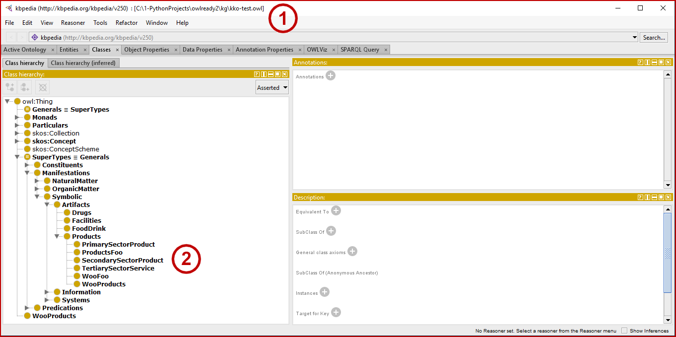
OK, so after saving we can inspect our new file to make sure that all of the class changes above are now accurately reflected in the formal ontology. Here is the class view for Products:

Example Markdown Cell in Edit Mode
Figure 1: Result of KKO Class Changes

We can see that our file now has the updated file name (1), and the added classes appear in the KKO ontology (2).

As the use of Protege proves, our changes have been written to our formal ontology correctly. If we so chose, we can now re-name back to our working file, and continue on with our work. Of course, after doing such checks beginning in our process or when we introduce new major wrinkles, we can gain confidence everything is working properly and skip labor-intensive checks as appropriate.

Additional Documentation

Owlready2 has relevant additional documentation, with examples, for:

NOTE: This article is part of the Cooking with Python and KBpedia series. See the CWPK listing for other articles in the series. KBpedia has its own Web site.
NOTE: This CWPK installment is available both as an online interactive file or as a direct download to use locally. Make sure and pick the correct installment number. For the online interactive option, pick the *.ipynb file. It may take a bit of time for the interactive option to load.
I am at best an amateur with Python. There are likely more efficient methods for coding these steps than what I provide. I encourage you to experiment — which is part of the fun of Python — and to notify me should you make improvements.

Posted by AI3's author, Mike Bergman Posted on August 21, 2020 at 10:46 am in CWPK, KBpedia, Semantic Web Tools | Comments (0)
The URI link reference to this post is: https://www.mkbergman.com/2350/cwpk-20-basic-knowledge-graph-management-i/
The URI to trackback this post is: https://www.mkbergman.com/2350/cwpk-20-basic-knowledge-graph-management-i/trackback/
Posted:August 20, 2020

Let’s Get Familiar with Some Basic owlready2 Commands

In our last installment of this Cooking with Python and KBpedia series, we learned some KBpedia terminology and loaded the main KBpedia knowledge graph file, kbpedia_reference_concepts.owl. (Remember, do NOT use the kbpedia_reference_concepts.n3 since owlready2 does not support the Notation3 syntax.) You will need to navigate back to that file location again. One of the aspects of working with Jupyter Notebook is that, once you leave the application, you must re-load your files again whenever you return to the application. As you also recall, it is also necessary to Run the cells in order for a given notebook to restore the states that each cell needs.

In today’s installment we will start to get familiar with some basic commands in owlready2, the API to our OWL2 ontologies. We will then apply these basic approaches to starting efforts to manage these ontologies, which begins with our next installment.

Load and Import the Ontologies

Which environment? The specific load routine you should choose below depends on whether you are using the online MyBinder service (the ‘raw’ version) or local files. See CWPK #17 for further details.

Local File Option

As we instructed in the last installment, the best practice is to provide names to absolute file addresses to make sure you are getting and loading the files you need. Again, in this instance, we call name this file main and we also add some code to verify the file was found by listing its contents:

main = 'C:/1-PythonProjects/kbpedia/sandbox/kbpedia_reference_concepts.owl'
with open(main) as fobj:                           
    for line in fobj:
        print (line)

After you shift+enter to execute the cell contents, or pick Run from the main menu, you will see a rather long file listing. To clear it from the screen, run Cell → All Output → Clear.

The KBpedia full ontology also depends on (‘imports’) two other files: the KBpedia upper ontology, KKO (kko.owl), and the SKOS language that we use for annotations (http://www.w3.org/2004/02/skos/core). The KBpedia full ontology also depends on (‘imports’) two other files: the KBpedia upper ontology, KKO (kko.owl), and the SKOS language that we use for annotations (http://www.w3.org/2004/02/skos/core). As we described in the prior CWPK installment, you will need to download the raw version of kko.owl, and store it in the same location as kbpedia_reference_concepts.owl downloaded in the prior installment. There is no need to download the skos file.

Again, we give names to their absolute file addresses, only this time we do not echo their file listings to screen:

kko_file = r'C:\1-PythonProjects\kbpedia\sandbox\kko.owl' 
skos_file = 'http://www.w3.org/2004/02/skos/core' 

Note one file (kko) is on disk and we use the native Windows file path (with backward slashes) by invoking the ‘r‘ (raw) command switch: r'C:\1-PythonProjects\kbpedia\sandbox\kko.owl'. The other skos file is found off of the Web.

MyBinder Option

If you are running this notebook online, do NOT run the above routines, since the load routines vary somewhat. Please use the following instructions.

main = 'https://raw.githubusercontent.com/Cognonto/CWPK/master/sandbox/builds/ontologies/kbpedia_reference_concepts.owl'

To view this file, run the next cell, otherwise, run the following cells to load all graphs.

import urllib.request 

for line in urllib.request.urlopen(main):
    print(line.decode('utf-8'), end='')
kko_file = 'https://raw.githubusercontent.com/Cognonto/CWPK/master/sandbox/builds/ontologies/kko.owl' 
skos_file = 'http://www.w3.org/2004/02/skos/core' 

Begin the Import

Now that our three files have been given logical names, we are ready to import them into our Jupyter Notebook. Run each of these cells (shift+enter) in sequence:

from owlready2 import *
onto = get_ontology(main).load()

The asterisk (*) after the import statement means that we want to load all modules in the owlready2 package. One of those functions is get_ontology. We have also given our main ontology the name of onto

skos = get_ontology(skos_file).load()
onto.imported_ontologies.append(skos) 
kko = get_ontology(kko_file).load()
onto.imported_ontologies.append(kko) 

We can also place all three commands into a single cell. Note, however, that if you run this consolidated command, that you will see double listings when you invoke print(onto.imported_ontologies) below. In other words, while there is no harm to loading a file again, you are better off only doing the consolidated alone or the three separate loads alone.

You can run the command below to see this behavior. You should then log off or Kernal → Restart & Clear Output and then only load one set before proceeding further.

from owlready2 import *
onto = get_ontology(main).load()

skos = get_ontology(skos_file).load()
onto.imported_ontologies.append(skos) 

kko = get_ontology(kko_file).load()
onto.imported_ontologies.append(kko)

Let’s now test to make sure the ontologies have been loaded OK by checking to see if the base IRIs for all graphs are recognized by the system:

print(onto.base_iri)
http://kbpedia.org/kbpedia/rc#
print(skos.base_iri)
print(kko.base_iri)

We can also confirm that the two additional ontologies have been properly imported:

print(onto.imported_ontologies)

Inspecting Ontology Contents

We can now start checking to see if the components of the ontologies have loaded properly. Let’s first check on the classes:

list(onto.classes())

Now, this listing above is interesting. You will see a few warning messages at the top of the listing. This is due to the fact that a very few KBpedia RCs share the same subClasses, making them essentially equivalent classes. The ones listed here are purposeful and do no harm; generally, however, you want to avoid such duplication.

Next, if you scroll down to the bottom you will see that the listing is actually truncated at the bottom with the [...] indicator. If you were to copy the output listing to an editor you would see there are exactly 1000 items in this list, the default limit for such listings when you first install Jupyter Python. But we know there are more than 58,000 RCs (classes) in the system. To see a complete listing we will need to make a change to our notebook’s configuration file.

Note: This option does not apply to the online MyBinder version.

First, you need to exit this notebook and at your command line create an IPython config file if you don’t already have one:

ipython profile create

Once generated, this config file can be found in your user’s directory (C:\Users\mike.ipython\profile_default\ipython_config.py in my case). Make sure and note the dot in the .ipython directory. Navigate to your appropriate directory and edit this config file to remove the comment for this line and to set the value to ‘0’:

c.PlainTextFormatter.max_seq_length = 0

(which, again, is set to 1000 by default.)

Restart your notebook instance after making this change and run the cells above again. You will now see the full listing of RCs in KBpedia. (A hat tip to StackOverflow for this snippet.)

But, hmmm, where are the classes from the kko and skos imports? All we are showing in this list are the RCs from the default ontology of main.

One of the interesting aspects of owlready2 is its use of what it calls ‘worlds’ to isolate given items into separate namespaces. This allows different projects to be held in memory at one time, including even different open and closed reasoning that may be applied. (A topic for a later installment.)

Now, it is the case that we loaded all three of our ontologies without specifying different ‘world’ namespaces. To see the three combined, let’s actually specify the ‘world’ that is currently active, which is called ‘default’ if not otherwise specified. Rather than our previous onto namespace, let’s now explicitly refer to this default:

list(default_world.classes()) 

Note the full IRI listings for the kko classes at the bottom of the listing. This signals a bit of a namespace recognition problem, that we will address in a few moments.

We can use this same dot approach of namespace.method for other components in our system. (See Additional Documentation below for a listing of such methods available in owlready2.)

In the two examples below we list the annotation properties for both the main (onto) and skos namespaces:

list(onto.annotation_properties())
list(skos.annotation_properties())

Now, one of the RCs we see in our listing is for Eutheria, the technical name for mammals. Using the same format as above we want to get a listing of its subclasses, but adding our rc. prefix in fact does not work:

list(rc.Eutheria.subclasses())

Hmmm, it is not immediately clear why we get the error that ‘rc‘ is not defined.

If we look at the KBpedia Web site we see, in fact, that our prefix to individual RCs is actually http://kbpedia.org/kko/rc/ with the trailing ‘/’. owlready2 documentation indicates it uses the ‘#’ sign as its default separator for vocabulary terms. Since our system uses the ‘/’, perhaps something got screwed up in how owlready2 recognizes our namespace.

One way to deal with this potential problem explicitly is to make a direct assignment for what the IRI prefix should be. We do so via this command, where we are directing the prefix ‘rc‘ to recognize our standard base IRI:

rc = onto.get_namespace('http://kbpedia.org/kko/rc/')

With this new namespace assignment, we run the command again:

list(rc.Eutheria.subclasses())

Voilà! We now have the proper registry of the namespace in our system.

Along with absolute file names that we reference via assigned names, it is also good practice to make sure that our namespaces are properly registered before beginning work with owlready2. (I may discover better tips as we move ahead that I will post when and if discovered.)

We can also check out the properties for this concept:

list(rc.Eutheria.get_class_properties())

And, pull out our definition for the concept:

print(rc.Eutheria.definition)

There is also the alternate IRI sytax for identifying a class, in this case to obtain all of the children, grandchildren, etc., of our Mammal concept (which produces a long list of mammals!):

IRIS['http://kbpedia.org/kko/rc/Mammal'].descendants() 

Since we have used the Python list method quite a bit, we can get direct assistance about the method with the standard command:

help(list)

We can also conduct searches of our RCs, including with wildcards (*) in either the pre or post positions:

onto.search(iri = "*Luggage*")

Another helpful command in owlready2 is to instruct the system what paths to search when it looks for referenced names:

onto_path.append("C:/1-PythonProjects/kbpedia/sandbox")

And, we can get a listing of all such paths registered:

list(onto_path)

Lastly, for this installment, we can close by saving the ontology we have been working on, being careful in this instance to give a different file name to prevent inadvertent overwriting of our initial input file:

onto.save(file = "C:/1-PythonProjects/kbpedia/sandbox/owl-test.owl", format = "rdfxml")

To properly exit the notebook, first pick File → Save and Checkpoint, then File → Close and Halt. This will return you to the main Jupyter files screen, from which you Quit and then close the tab. Return to the command window and finish shutting down the service with ctrl+c. That will return you to the command prompt, from which you may again start up a ‘Jupyter Notebook‘ instance.

Additional Documentation

Here is a listing of owlready2 ontology methods.

NOTE: This article is part of the Cooking with Python and KBpedia series. See the CWPK listing for other articles in the series. KBpedia has its own Web site.
NOTE: This CWPK installment is available both as an online interactive file or as a direct download to use locally. Make sure and pick the correct installment number. For the online interactive option, pick the *.ipynb file. It may take a bit of time for the interactive option to load.
I am at best an amateur with Python. There are likely more efficient methods for coding these steps than what I provide. I encourage you to experiment — which is part of the fun of Python — and to notify me should you make improvements.

Posted by AI3's author, Mike Bergman Posted on August 20, 2020 at 10:38 am in CWPK, KBpedia, Semantic Web Tools | Comments (0)
The URI link reference to this post is: https://www.mkbergman.com/2349/cwpk-19-exploring-the-api-to-owl/
The URI to trackback this post is: https://www.mkbergman.com/2349/cwpk-19-exploring-the-api-to-owl/trackback/